![]()
01. Neural Network Regression with TensorFlow
There are many definitions for a regression problem but in our case, we're going to simplify it to be: predicting a number.
For example, you might want to:
- Predict the selling price of houses given information about them (such as number of rooms, size, number of bathrooms).
- Predict the coordinates of a bounding box of an item in an image.
- Predict the cost of medical insurance for an individual given their demographics (age, sex, gender, race).
In this notebook, we're going to set the foundations for how you can take a sample of inputs (this is your data), build a neural network to discover patterns in those inputs and then make a prediction (in the form of a number) based on those inputs.
What we're going to cover
Specifically, we're going to go through doing the following with TensorFlow:
- Architecture of a regression model
- Input shapes and output shapes
X: features/data (inputs)y: labels (outputs)
- Creating custom data to view and fit
- Steps in modelling
- Creating a model
- Compiling a model
- Defining a loss function
- Setting up an optimizer
- Creating evaluation metrics
- Fitting a model (getting it to find patterns in our data)
- Evaluating a model
- Visualizng the model ("visualize, visualize, visualize")
- Looking at training curves
- Compare predictions to ground truth (using our evaluation metrics)
- Saving a model (so we can use it later)
- Loading a model
Don't worry if none of these make sense now, we're going to go through each.
How you can use this notebook
You can read through the descriptions and the code (it should all run), but there's a better option.
Write all of the code yourself.
Yes. I'm serious. Create a new notebook, and rewrite each line by yourself. Investigate it, see if you can break it, why does it break?
You don't have to write the text descriptions but writing the code yourself is a great way to get hands-on experience.
Don't worry if you make mistakes, we all do. The way to get better and make less mistakes is to write more code.
Typical architecture of a regresison neural network
The word typical is on purpose.
Why?
Because there are many different ways (actually, there's almost an infinite number of ways) to write neural networks.
But the following is a generic setup for ingesting a collection of numbers, finding patterns in them and then outputting some kind of target number.
Yes, the previous sentence is vague but we'll see this in action shortly.
| Hyperparameter | Typical value |
|---|---|
| Input layer shape | Same shape as number of features (e.g. 3 for # bedrooms, # bathrooms, # car spaces in housing price prediction) |
| Hidden layer(s) | Problem specific, minimum = 1, maximum = unlimited |
| Neurons per hidden layer | Problem specific, generally 10 to 100 |
| Output layer shape | Same shape as desired prediction shape (e.g. 1 for house price) |
| Hidden activation | Usually ReLU (rectified linear unit) |
| Output activation | None, ReLU, logistic/tanh |
| Loss function | MSE (mean square error) or MAE (mean absolute error)/Huber (combination of MAE/MSE) if outliers |
| Optimizer | SGD (stochastic gradient descent), Adam |
Table 1: Typical architecture of a regression network. Source: Adapted from page 293 of Hands-On Machine Learning with Scikit-Learn, Keras & TensorFlow Book by Aurélien Géron
Again, if you're new to neural networks and deep learning in general, much of the above table won't make sense. But don't worry, we'll be getting hands-on with all of it soon.
🔑 Note: A hyperparameter in machine learning is something a data analyst or developer can set themselves, where as a parameter usually describes something a model learns on its own (a value not explicitly set by an analyst).
Okay, enough talk, let's get started writing code.
To use TensorFlow, we'll import it as the common alias tf (short for TensorFlow).
import tensorflow as tf
print(tf.__version__) # check the version (should be 2.x+)

import datetime
print(f"Notebook last run (end-to-end): {datetime.datetime.now()}")
2.12.0
Notebook last run (end-to-end): 2023-05-07 23:10:01.302908
Creating data to view and fit
Since we're working on a regression problem (predicting a number) let's create some linear data (a straight line) to model.
import numpy as np
import matplotlib.pyplot as plt

# Create features
X = np.array([-7.0, -4.0, -1.0, 2.0, 5.0, 8.0, 11.0, 14.0])

# Create labels
y = np.array([3.0, 6.0, 9.0, 12.0, 15.0, 18.0, 21.0, 24.0])

# Visualize it
plt.scatter(X, y);

Before we do any modelling, can you calculate the pattern between X and y?
For example, say I asked you, based on this data what the y value would be if X was 17.0?
Or how about if X was -10.0?
This kind of pattern discovery is the essence of what we'll be building neural networks to do for us.
Regression input shapes and output shapes
One of the most important concepts when working with neural networks are the input and output shapes.
The input shape is the shape of your data that goes into the model.
The output shape is the shape of your data you want to come out of your model.
These will differ depending on the problem you're working on.
Neural networks accept numbers and output numbers. These numbers are typically represented as tensors (or arrays).
Before, we created data using NumPy arrays, but we could do the same with tensors.
# Example input and output shapes of a regression model
house_info = tf.constant(["bedroom", "bathroom", "garage"])
house_price = tf.constant([939700])
house_info, house_price
(<tf.Tensor: shape=(3,), dtype=string, numpy=array([b'bedroom', b'bathroom', b'garage'], dtype=object)>,
 <tf.Tensor: shape=(1,), dtype=int32, numpy=array([939700], dtype=int32)>)
house_info.shape
TensorShape([3])
import numpy as np
import matplotlib.pyplot as plt

# Create features (using tensors)
X = tf.constant([-7.0, -4.0, -1.0, 2.0, 5.0, 8.0, 11.0, 14.0])

# Create labels (using tensors)
y = tf.constant([3.0, 6.0, 9.0, 12.0, 15.0, 18.0, 21.0, 24.0])

# Visualize it
plt.scatter(X, y);
Our goal here will be to use X to predict y.
So our input will be X and our output will be y.
Knowing this, what do you think our input and output shapes will be?
Let's take a look.
# Take a single example of X
input_shape = X[0].shape

# Take a single example of y
output_shape = y[0].shape

input_shape, output_shape # these are both scalars (no shape)
(TensorShape([]), TensorShape([]))
Huh?
From this it seems our inputs and outputs have no shape?
How could that be?
It's because no matter what kind of data we pass to our model, it's always going to take as input and return as output some kind of tensor.
But in our case because of our dataset (only 2 small lists of numbers), we're looking at a special kind of tensor, more specifically a rank 0 tensor or a scalar.
# Let's take a look at the single examples invidually
X[0], y[0]
(<tf.Tensor: shape=(), dtype=float32, numpy=-7.0>,
 <tf.Tensor: shape=(), dtype=float32, numpy=3.0>)
In our case, we're trying to build a model to predict the pattern between X[0] equalling -7.0 and y[0] equalling 3.0.
So now we get our answer, we're trying to use 1 X value to predict 1 y value.
You might be thinking, "this seems pretty complicated for just predicting a straight line...".
And you'd be right.
But the concepts we're covering here, the concepts of input and output shapes to a model are fundamental.
In fact, they're probably two of the things you'll spend the most time on when you work with neural networks: making sure your input and outputs are in the correct shape.
If it doesn't make sense now, we'll see plenty more examples later on (soon you'll notice the input and output shapes can be almost anything you can imagine).
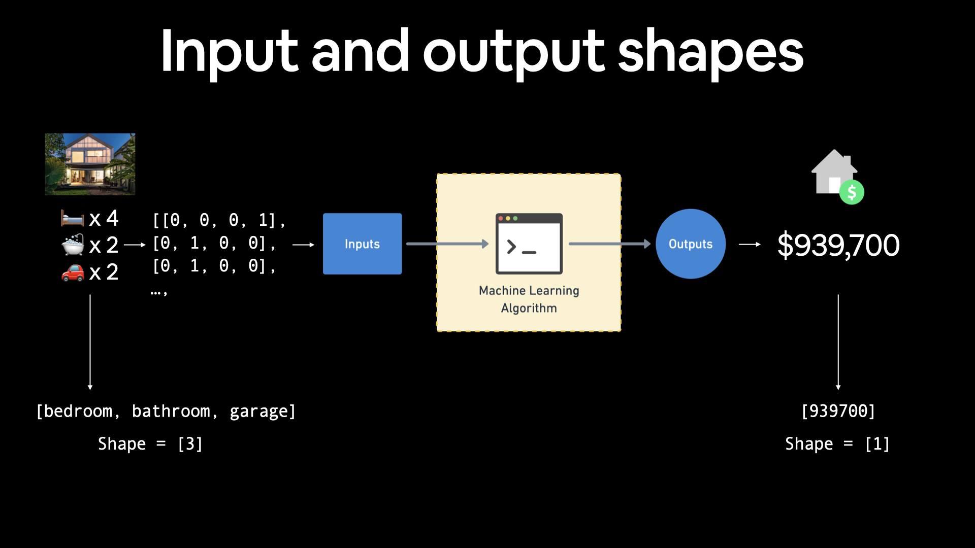 If you were working on building a machine learning algorithm for predicting housing prices, your inputs may be number of bedrooms, number of bathrooms and number of garages, giving you an input shape of 3 (3 different features). And since you're trying to predict the price of the house, your output shape would be 1.
Steps in modelling with TensorFlow
Now we know what data we have as well as the input and output shapes, let's see how we'd build a neural network to model it.
In TensorFlow, there are typically 3 fundamental steps to creating and training a model.
- Creating a model - piece together the layers of a neural network yourself (using the Functional or Sequential API) or import a previously built model (known as transfer learning).
- Compiling a model - defining how a models performance should be measured (loss/metrics) as well as defining how it should improve (optimizer).
- Fitting a model - letting the model try to find patterns in the data (how does
Xget toy).
Let's see these in action using the Keras Sequential API to build a model for our regression data. And then we'll step through each.
Note: If you're using TensorFlow 2.7.0+, the
fit()function no longer upscales input data to go from(batch_size, )to(batch_size, 1). To fix this, you'll need to expand the dimension of input data usingtf.expand_dims(input_data, axis=-1).In our case, this means instead of using
model.fit(X, y, epochs=5), usemodel.fit(tf.expand_dims(X, axis=-1), y, epochs=5).
# Set random seed
tf.random.set_seed(42)

# Create a model using the Sequential API
model = tf.keras.Sequential([
  tf.keras.layers.Dense(1)
])

# Compile the model
model.compile(loss=tf.keras.losses.mae, # mae is short for mean absolute error
              optimizer=tf.keras.optimizers.SGD(), # SGD is short for stochastic gradient descent
              metrics=["mae"])

# Fit the model
# model.fit(X, y, epochs=5) # this will break with TensorFlow 2.7.0+
model.fit(tf.expand_dims(X, axis=-1), y, epochs=5)
Epoch 1/5
1/1 [==============================] - 6s 6s/step - loss: 19.2976 - mae: 19.2976
Epoch 2/5
1/1 [==============================] - 0s 18ms/step - loss: 19.0164 - mae: 19.0164
Epoch 3/5
1/1 [==============================] - 0s 12ms/step - loss: 18.7351 - mae: 18.7351
Epoch 4/5
1/1 [==============================] - 0s 13ms/step - loss: 18.4539 - mae: 18.4539
Epoch 5/5
1/1 [==============================] - 0s 13ms/step - loss: 18.1726 - mae: 18.1726
<keras.callbacks.History at 0x7f00663d2680>
Boom!
We've just trained a model to figure out the patterns between X and y.
How do you think it went?
# Check out X and y
X, y
(<tf.Tensor: shape=(8,), dtype=float32, numpy=array([-7., -4., -1.,  2.,  5.,  8., 11., 14.], dtype=float32)>,
 <tf.Tensor: shape=(8,), dtype=float32, numpy=array([ 3.,  6.,  9., 12., 15., 18., 21., 24.], dtype=float32)>)
What do you think the outcome should be if we passed our model an X value of 17.0?
# Make a prediction with the model
model.predict([17.0])
1/1 [==============================] - 0s 115ms/step
array([[-16.701845]], dtype=float32)
It doesn't go very well... it should've output something close to 27.0.
🤔 Question: What's Keras? I thought we were working with TensorFlow but every time we write TensorFlow code,
kerascomes aftertf(e.g.tf.keras.layers.Dense())?
Before TensorFlow 2.0+, Keras was an API designed to be able to build deep learning models with ease. Since TensorFlow 2.0+, its functionality has been tightly integrated within the TensorFlow library.
Improving a model
How do you think you'd improve upon our current model?
If you guessed by tweaking some of the things we did above, you'd be correct.
To improve our model, we alter almost every part of the 3 steps we went through before.
- Creating a model - here you might want to add more layers, increase the number of hidden units (also called neurons) within each layer, change the activation functions of each layer.
- Compiling a model - you might want to choose optimization function or perhaps change the learning rate of the optimization function.
- Fitting a model - perhaps you could fit a model for more epochs (leave it training for longer) or on more data (give the model more examples to learn from).
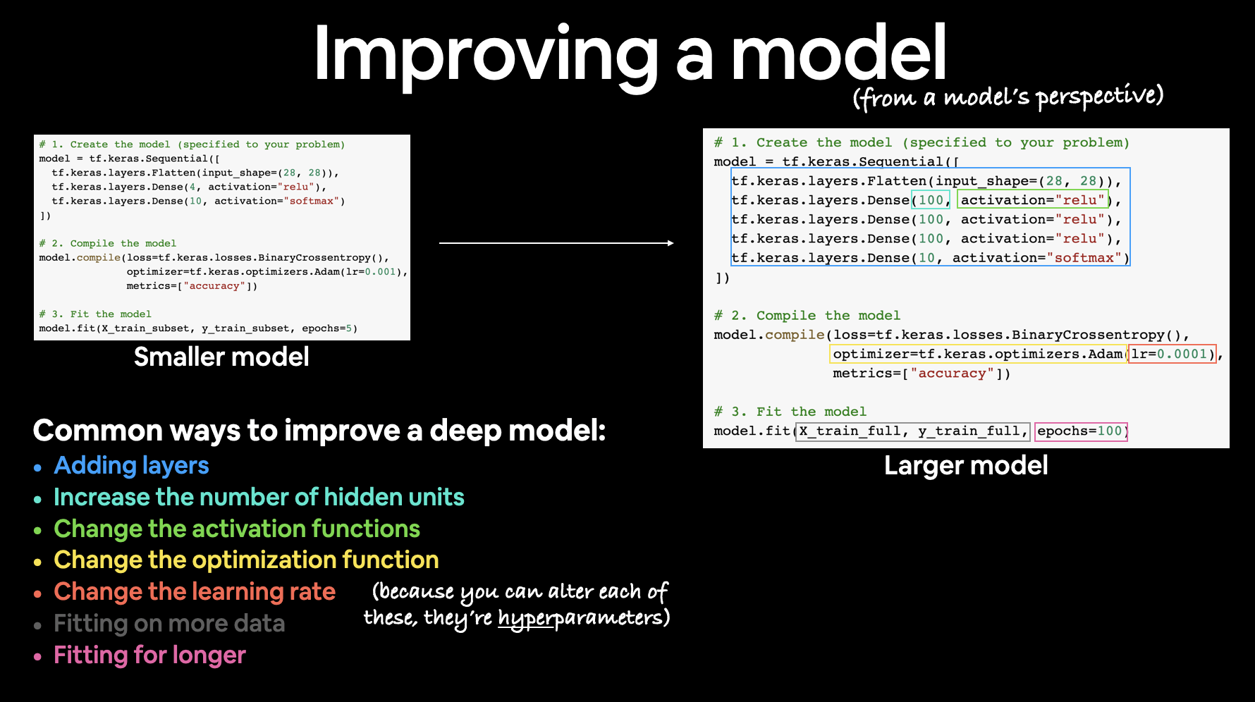 There are many different ways to potentially improve a neural network. Some of the most common include: increasing the number of layers (making the network deeper), increasing the number of hidden units (making the network wider) and changing the learning rate. Because these values are all human-changeable, they're referred to as hyperparameters) and the practice of trying to find the best hyperparameters is referred to as hyperparameter tuning.
Woah. We just introduced a bunch of possible steps. The important thing to remember is how you alter each of these will depend on the problem you're working on.
And the good thing is, over the next few problems, we'll get hands-on with all of them.
For now, let's keep it simple, all we'll do is train our model for longer (everything else will stay the same).
# Set random seed
tf.random.set_seed(42)

# Create a model (same as above)
model = tf.keras.Sequential([
  tf.keras.layers.Dense(1)
])

# Compile model (same as above)
model.compile(loss=tf.keras.losses.mae,
              optimizer=tf.keras.optimizers.SGD(),
              metrics=["mae"])

# Fit model (this time we'll train for longer)
model.fit(tf.expand_dims(X, axis=-1), y, epochs=100) # train for 100 epochs not 10
Epoch 1/100
1/1 [==============================] - 1s 604ms/step - loss: 12.9936 - mae: 12.9936
Epoch 2/100
1/1 [==============================] - 0s 14ms/step - loss: 12.8611 - mae: 12.8611
Epoch 3/100
1/1 [==============================] - 0s 16ms/step - loss: 12.7286 - mae: 12.7286
Epoch 4/100
1/1 [==============================] - 0s 16ms/step - loss: 12.5961 - mae: 12.5961
Epoch 5/100
1/1 [==============================] - 0s 15ms/step - loss: 12.4636 - mae: 12.4636
Epoch 6/100
1/1 [==============================] - 0s 15ms/step - loss: 12.3311 - mae: 12.3311
Epoch 7/100
1/1 [==============================] - 0s 15ms/step - loss: 12.1986 - mae: 12.1986
Epoch 8/100
1/1 [==============================] - 0s 16ms/step - loss: 12.0661 - mae: 12.0661
Epoch 9/100
1/1 [==============================] - 0s 13ms/step - loss: 11.9336 - mae: 11.9336
Epoch 10/100
1/1 [==============================] - 0s 14ms/step - loss: 11.8011 - mae: 11.8011
Epoch 11/100
1/1 [==============================] - 0s 12ms/step - loss: 11.6686 - mae: 11.6686
Epoch 12/100
1/1 [==============================] - 0s 13ms/step - loss: 11.5361 - mae: 11.5361
Epoch 13/100
1/1 [==============================] - 0s 13ms/step - loss: 11.4036 - mae: 11.4036
Epoch 14/100
1/1 [==============================] - 0s 13ms/step - loss: 11.2711 - mae: 11.2711
Epoch 15/100
1/1 [==============================] - 0s 13ms/step - loss: 11.1386 - mae: 11.1386
Epoch 16/100
1/1 [==============================] - 0s 12ms/step - loss: 11.0061 - mae: 11.0061
Epoch 17/100
1/1 [==============================] - 0s 12ms/step - loss: 10.8736 - mae: 10.8736
Epoch 18/100
1/1 [==============================] - 0s 12ms/step - loss: 10.7411 - mae: 10.7411
Epoch 19/100
1/1 [==============================] - 0s 12ms/step - loss: 10.6086 - mae: 10.6086
Epoch 20/100
1/1 [==============================] - 0s 12ms/step - loss: 10.4761 - mae: 10.4761
Epoch 21/100
1/1 [==============================] - 0s 12ms/step - loss: 10.3436 - mae: 10.3436
Epoch 22/100
1/1 [==============================] - 0s 12ms/step - loss: 10.2111 - mae: 10.2111
Epoch 23/100
1/1 [==============================] - 0s 18ms/step - loss: 10.0786 - mae: 10.0786
Epoch 24/100
1/1 [==============================] - 0s 10ms/step - loss: 9.9461 - mae: 9.9461
Epoch 25/100
1/1 [==============================] - 0s 9ms/step - loss: 9.8136 - mae: 9.8136
Epoch 26/100
1/1 [==============================] - 0s 10ms/step - loss: 9.6811 - mae: 9.6811
Epoch 27/100
1/1 [==============================] - 0s 10ms/step - loss: 9.5486 - mae: 9.5486
Epoch 28/100
1/1 [==============================] - 0s 10ms/step - loss: 9.4161 - mae: 9.4161
Epoch 29/100
1/1 [==============================] - 0s 11ms/step - loss: 9.2836 - mae: 9.2836
Epoch 30/100
1/1 [==============================] - 0s 11ms/step - loss: 9.1511 - mae: 9.1511
Epoch 31/100
1/1 [==============================] - 0s 9ms/step - loss: 9.0186 - mae: 9.0186
Epoch 32/100
1/1 [==============================] - 0s 9ms/step - loss: 8.8861 - mae: 8.8861
Epoch 33/100
1/1 [==============================] - 0s 10ms/step - loss: 8.7536 - mae: 8.7536
Epoch 34/100
1/1 [==============================] - 0s 10ms/step - loss: 8.6211 - mae: 8.6211
Epoch 35/100
1/1 [==============================] - 0s 12ms/step - loss: 8.4886 - mae: 8.4886
Epoch 36/100
1/1 [==============================] - 0s 10ms/step - loss: 8.3561 - mae: 8.3561
Epoch 37/100
1/1 [==============================] - 0s 9ms/step - loss: 8.2236 - mae: 8.2236
Epoch 38/100
1/1 [==============================] - 0s 8ms/step - loss: 8.0911 - mae: 8.0911
Epoch 39/100
1/1 [==============================] - 0s 10ms/step - loss: 7.9586 - mae: 7.9586
Epoch 40/100
1/1 [==============================] - 0s 9ms/step - loss: 7.8261 - mae: 7.8261
Epoch 41/100
1/1 [==============================] - 0s 9ms/step - loss: 7.6936 - mae: 7.6936
Epoch 42/100
1/1 [==============================] - 0s 9ms/step - loss: 7.5611 - mae: 7.5611
Epoch 43/100
1/1 [==============================] - 0s 9ms/step - loss: 7.4286 - mae: 7.4286
Epoch 44/100
1/1 [==============================] - 0s 9ms/step - loss: 7.2961 - mae: 7.2961
Epoch 45/100
1/1 [==============================] - 0s 9ms/step - loss: 7.1700 - mae: 7.1700
Epoch 46/100
1/1 [==============================] - 0s 9ms/step - loss: 7.1644 - mae: 7.1644
Epoch 47/100
1/1 [==============================] - 0s 9ms/step - loss: 7.1588 - mae: 7.1588
Epoch 48/100
1/1 [==============================] - 0s 9ms/step - loss: 7.1531 - mae: 7.1531
Epoch 49/100
1/1 [==============================] - 0s 10ms/step - loss: 7.1475 - mae: 7.1475
Epoch 50/100
1/1 [==============================] - 0s 10ms/step - loss: 7.1419 - mae: 7.1419
Epoch 51/100
1/1 [==============================] - 0s 8ms/step - loss: 7.1363 - mae: 7.1363
Epoch 52/100
1/1 [==============================] - 0s 9ms/step - loss: 7.1306 - mae: 7.1306
Epoch 53/100
1/1 [==============================] - 0s 9ms/step - loss: 7.1250 - mae: 7.1250
Epoch 54/100
1/1 [==============================] - 0s 9ms/step - loss: 7.1194 - mae: 7.1194
Epoch 55/100
1/1 [==============================] - 0s 11ms/step - loss: 7.1138 - mae: 7.1138
Epoch 56/100
1/1 [==============================] - 0s 10ms/step - loss: 7.1081 - mae: 7.1081
Epoch 57/100
1/1 [==============================] - 0s 9ms/step - loss: 7.1025 - mae: 7.1025
Epoch 58/100
1/1 [==============================] - 0s 9ms/step - loss: 7.0969 - mae: 7.0969
Epoch 59/100
1/1 [==============================] - 0s 9ms/step - loss: 7.0913 - mae: 7.0913
Epoch 60/100
1/1 [==============================] - 0s 9ms/step - loss: 7.0856 - mae: 7.0856
Epoch 61/100
1/1 [==============================] - 0s 9ms/step - loss: 7.0800 - mae: 7.0800
Epoch 62/100
1/1 [==============================] - 0s 8ms/step - loss: 7.0744 - mae: 7.0744
Epoch 63/100
1/1 [==============================] - 0s 9ms/step - loss: 7.0688 - mae: 7.0688
Epoch 64/100
1/1 [==============================] - 0s 8ms/step - loss: 7.0631 - mae: 7.0631
Epoch 65/100
1/1 [==============================] - 0s 9ms/step - loss: 7.0575 - mae: 7.0575
Epoch 66/100
1/1 [==============================] - 0s 9ms/step - loss: 7.0519 - mae: 7.0519
Epoch 67/100
1/1 [==============================] - 0s 10ms/step - loss: 7.0463 - mae: 7.0463
Epoch 68/100
1/1 [==============================] - 0s 11ms/step - loss: 7.0406 - mae: 7.0406
Epoch 69/100
1/1 [==============================] - 0s 10ms/step - loss: 7.0350 - mae: 7.0350
Epoch 70/100
1/1 [==============================] - 0s 9ms/step - loss: 7.0294 - mae: 7.0294
Epoch 71/100
1/1 [==============================] - 0s 9ms/step - loss: 7.0238 - mae: 7.0238
Epoch 72/100
1/1 [==============================] - 0s 9ms/step - loss: 7.0181 - mae: 7.0181
Epoch 73/100
1/1 [==============================] - 0s 9ms/step - loss: 7.0125 - mae: 7.0125
Epoch 74/100
1/1 [==============================] - 0s 9ms/step - loss: 7.0069 - mae: 7.0069
Epoch 75/100
1/1 [==============================] - 0s 10ms/step - loss: 7.0013 - mae: 7.0013
Epoch 76/100
1/1 [==============================] - 0s 10ms/step - loss: 6.9956 - mae: 6.9956
Epoch 77/100
1/1 [==============================] - 0s 10ms/step - loss: 6.9900 - mae: 6.9900
Epoch 78/100
1/1 [==============================] - 0s 10ms/step - loss: 6.9844 - mae: 6.9844
Epoch 79/100
1/1 [==============================] - 0s 9ms/step - loss: 6.9788 - mae: 6.9788
Epoch 80/100
1/1 [==============================] - 0s 9ms/step - loss: 6.9731 - mae: 6.9731
Epoch 81/100
1/1 [==============================] - 0s 10ms/step - loss: 6.9675 - mae: 6.9675
Epoch 82/100
1/1 [==============================] - 0s 9ms/step - loss: 6.9619 - mae: 6.9619
Epoch 83/100
1/1 [==============================] - 0s 9ms/step - loss: 6.9563 - mae: 6.9563
Epoch 84/100
1/1 [==============================] - 0s 8ms/step - loss: 6.9506 - mae: 6.9506
Epoch 85/100
1/1 [==============================] - 0s 9ms/step - loss: 6.9450 - mae: 6.9450
Epoch 86/100
1/1 [==============================] - 0s 9ms/step - loss: 6.9394 - mae: 6.9394
Epoch 87/100
1/1 [==============================] - 0s 9ms/step - loss: 6.9338 - mae: 6.9338
Epoch 88/100
1/1 [==============================] - 0s 9ms/step - loss: 6.9281 - mae: 6.9281
Epoch 89/100
1/1 [==============================] - 0s 10ms/step - loss: 6.9225 - mae: 6.9225
Epoch 90/100
1/1 [==============================] - 0s 9ms/step - loss: 6.9169 - mae: 6.9169
Epoch 91/100
1/1 [==============================] - 0s 9ms/step - loss: 6.9113 - mae: 6.9113
Epoch 92/100
1/1 [==============================] - 0s 10ms/step - loss: 6.9056 - mae: 6.9056
Epoch 93/100
1/1 [==============================] - 0s 8ms/step - loss: 6.9000 - mae: 6.9000
Epoch 94/100
1/1 [==============================] - 0s 11ms/step - loss: 6.8944 - mae: 6.8944
Epoch 95/100
1/1 [==============================] - 0s 9ms/step - loss: 6.8888 - mae: 6.8888
Epoch 96/100
1/1 [==============================] - 0s 9ms/step - loss: 6.8831 - mae: 6.8831
Epoch 97/100
1/1 [==============================] - 0s 10ms/step - loss: 6.8775 - mae: 6.8775
Epoch 98/100
1/1 [==============================] - 0s 15ms/step - loss: 6.8719 - mae: 6.8719
Epoch 99/100
1/1 [==============================] - 0s 10ms/step - loss: 6.8663 - mae: 6.8663
Epoch 100/100
1/1 [==============================] - 0s 9ms/step - loss: 6.8606 - mae: 6.8606
<keras.callbacks.History at 0x7f0065eabcd0>
You might've noticed the loss value decrease from before (and keep decreasing as the number of epochs gets higher).
What do you think this means for when we make a prediction with our model?
How about we try predict on 17.0 again?
# Remind ourselves of what X and y are
X, y
(<tf.Tensor: shape=(8,), dtype=float32, numpy=array([-7., -4., -1.,  2.,  5.,  8., 11., 14.], dtype=float32)>,
 <tf.Tensor: shape=(8,), dtype=float32, numpy=array([ 3.,  6.,  9., 12., 15., 18., 21., 24.], dtype=float32)>)
# Try and predict what y would be if X was 17.0
model.predict([17.0]) # the right answer is 27.0 (y = X + 10)
1/1 [==============================] - 0s 61ms/step
array([[29.499516]], dtype=float32)
Much better!
We got closer this time. But we could still be better.
Now we've trained a model, how could we evaluate it?
Evaluating a model
A typical workflow you'll go through when building neural networks is:
Build a model -> evaluate it -> build (tweak) a model -> evaulate it -> build (tweak) a model -> evaluate it...
The tweaking comes from maybe not building a model from scratch but adjusting an existing one.
Visualize, visualize, visualize
When it comes to evaluation, you'll want to remember the words: "visualize, visualize, visualize."
This is because you're probably better looking at something (doing) than you are thinking about something.
It's a good idea to visualize:
- The data - what data are you working with? What does it look like?
- The model itself - what does the architecture look like? What are the different shapes?
- The training of a model - how does a model perform while it learns?
- The predictions of a model - how do the predictions of a model line up against the ground truth (the original labels)?
Let's start by visualizing the model.
But first, we'll create a little bit of a bigger dataset and a new model we can use (it'll be the same as before, but the more practice the better).
# Make a bigger dataset
X = np.arange(-100, 100, 4)
X
array([-100,  -96,  -92,  -88,  -84,  -80,  -76,  -72,  -68,  -64,  -60,
        -56,  -52,  -48,  -44,  -40,  -36,  -32,  -28,  -24,  -20,  -16,
        -12,   -8,   -4,    0,    4,    8,   12,   16,   20,   24,   28,
         32,   36,   40,   44,   48,   52,   56,   60,   64,   68,   72,
         76,   80,   84,   88,   92,   96])
# Make labels for the dataset (adhering to the same pattern as before)
y = np.arange(-90, 110, 4)
y
array([-90, -86, -82, -78, -74, -70, -66, -62, -58, -54, -50, -46, -42,
       -38, -34, -30, -26, -22, -18, -14, -10,  -6,  -2,   2,   6,  10,
        14,  18,  22,  26,  30,  34,  38,  42,  46,  50,  54,  58,  62,
        66,  70,  74,  78,  82,  86,  90,  94,  98, 102, 106])
Since $y=X+10$, we could make the labels like so:
# Same result as above
y = X + 10
y
array([-90, -86, -82, -78, -74, -70, -66, -62, -58, -54, -50, -46, -42,
       -38, -34, -30, -26, -22, -18, -14, -10,  -6,  -2,   2,   6,  10,
        14,  18,  22,  26,  30,  34,  38,  42,  46,  50,  54,  58,  62,
        66,  70,  74,  78,  82,  86,  90,  94,  98, 102, 106])
Split data into training/test set
One of the other most common and important steps in a machine learning project is creating a training and test set (and when required, a validation set).
Each set serves a specific purpose:
- Training set - the model learns from this data, which is typically 70-80% of the total data available (like the course materials you study during the semester).
- Validation set - the model gets tuned on this data, which is typically 10-15% of the total data available (like the practice exam you take before the final exam).
- Test set - the model gets evaluated on this data to test what it has learned, it's typically 10-15% of the total data available (like the final exam you take at the end of the semester).
For now, we'll just use a training and test set, this means we'll have a dataset for our model to learn on as well as be evaluated on.
We can create them by splitting our X and y arrays.
🔑 Note: When dealing with real-world data, this step is typically done right at the start of a project (the test set should always be kept separate from all other data). We want our model to learn on training data and then evaluate it on test data to get an indication of how well it generalizes to unseen examples.
# Check how many samples we have
len(X)
50
# Split data into train and test sets
X_train = X[:40] # first 40 examples (80% of data)
y_train = y[:40]

X_test = X[40:] # last 10 examples (20% of data)
y_test = y[40:]

len(X_train), len(X_test)
(40, 10)
Visualizing the data
Now we've got our training and test data, it's a good idea to visualize it.
Let's plot it with some nice colours to differentiate what's what.
plt.figure(figsize=(10, 7))
# Plot training data in blue
plt.scatter(X_train, y_train, c='b', label='Training data')
# Plot test data in green
plt.scatter(X_test, y_test, c='g', label='Testing data')
# Show the legend
plt.legend();

Beautiful! Any time you can visualize your data, your model, your anything, it's a good idea.
With this graph in mind, what we'll be trying to do is build a model which learns the pattern in the blue dots (X_train) to draw the green dots (X_test).
Time to build a model. We'll make the exact same one from before (the one we trained for longer).
# Set random seed
tf.random.set_seed(42)

# Create a model (same as above)
model = tf.keras.Sequential([
  tf.keras.layers.Dense(1)
])

# Compile model (same as above)
model.compile(loss=tf.keras.losses.mae,
              optimizer=tf.keras.optimizers.SGD(),
              metrics=["mae"])

# Fit model (same as above)
#model.fit(X_train, y_train, epochs=100) # commented out on purpose (not fitting it just yet)
Visualizing the model
After you've built a model, you might want to take a look at it (especially if you haven't built many before).
You can take a look at the layers and shapes of your model by calling summary() on it.
🔑 Note: Visualizing a model is particularly helpful when you run into input and output shape mismatches.
# Doesn't work (model not fit/built)
model.summary()
---------------------------------------------------------------------------
ValueError                                Traceback (most recent call last)
<ipython-input-22-7d09d31d4e66> in <cell line: 2>()
      1 # Doesn't work (model not fit/built)
----> 2 model.summary()

/usr/local/lib/python3.10/dist-packages/keras/engine/training.py in summary(self, line_length, positions, print_fn, expand_nested, show_trainable, layer_range)
   3227         """
   3228         if not self.built:
-> 3229             raise ValueError(
   3230                 "This model has not yet been built. "
   3231                 "Build the model first by calling `build()` or by calling "

ValueError: This model has not yet been built. Build the model first by calling `build()` or by calling the model on a batch of data.
Ahh, the cell above errors because we haven't fit or built our model.
We also haven't told it what input shape it should be expecting.
Remember above, how we discussed the input shape was just one number?
We can let our model know the input shape of our data using the input_shape parameter to the first layer (usually if input_shape isn't defined, Keras tries to figure it out automatically).
# Set random seed
tf.random.set_seed(42)

# Create a model (same as above)
model = tf.keras.Sequential([
  tf.keras.layers.Dense(1, input_shape=[1]) # define the input_shape to our model
])

# Compile model (same as above)
model.compile(loss=tf.keras.losses.mae,
              optimizer=tf.keras.optimizers.SGD(),
              metrics=["mae"])
# This will work after specifying the input shape
model.summary()
Model: "sequential_3"
_________________________________________________________________
 Layer (type)                Output Shape              Param #
=================================================================
 dense_3 (Dense)             (None, 1)                 2

=================================================================
Total params: 2
Trainable params: 2
Non-trainable params: 0
_________________________________________________________________
Calling summary() on our model shows us the layers it contains, the output shape and the number of parameters.
- Total params - total number of parameters in the model.
- Trainable parameters - these are the parameters (patterns) the model can update as it trains.
- Non-trainable parameters - these parameters aren't updated during training (this is typical when you bring in the already learned patterns from other models during transfer learning).
📖 Resource: For a more in-depth overview of the trainable parameters within a layer, check out MIT's introduction to deep learning video.
🛠 Exercise: Try playing around with the number of hidden units in the
Denselayer (e.g.Dense(2),Dense(3)). How does this change the Total/Trainable params? Investigate what's causing the change.
For now, all you need to think about these parameters is that their learnable patterns in the data.
Let's fit our model to the training data.
# Fit the model to the training data
model.fit(X_train, y_train, epochs=100, verbose=0) # verbose controls how much gets output
<keras.callbacks.History at 0x7f0065dd80d0>
# Check the model summary
model.summary()
Model: "sequential_3"
_________________________________________________________________
 Layer (type)                Output Shape              Param #
=================================================================
 dense_3 (Dense)             (None, 1)                 2

=================================================================
Total params: 2
Trainable params: 2
Non-trainable params: 0
_________________________________________________________________
Alongside summary, you can also view a 2D plot of the model using plot_model().
from tensorflow.keras.utils import plot_model

plot_model(model, show_shapes=True)

In our case, the model we used only has an input and an output but visualizing more complicated models can be very helpful for debugging.
Visualizing the predictions
Now we've got a trained model, let's visualize some predictions.
To visualize predictions, it's always a good idea to plot them against the ground truth labels.
Often you'll see this in the form of y_test vs. y_pred (ground truth vs. predictions).
First, we'll make some predictions on the test data (X_test), remember the model has never seen the test data.
# Make predictions
y_preds = model.predict(X_test)
1/1 [==============================] - 0s 45ms/step
# View the predictions
y_preds
array([[44.544697],
       [47.427135],
       [50.309574],
       [53.192013],
       [56.07445 ],
       [58.95689 ],
       [61.839325],
       [64.72176 ],
       [67.60421 ],
       [70.48664 ]], dtype=float32)
Okay, we get a list of numbers but how do these compare to the ground truth labels?
Let's build a plotting function to find out.
🔑 Note: If you think you're going to be visualizing something a lot, it's a good idea to functionize it so you can use it later.
def plot_predictions(train_data=X_train,
                     train_labels=y_train,
                     test_data=X_test,
                     test_labels=y_test,
                     predictions=y_preds):
  """
  Plots training data, test data and compares predictions.
  """
  plt.figure(figsize=(10, 7))
  # Plot training data in blue
  plt.scatter(train_data, train_labels, c="b", label="Training data")
  # Plot test data in green
  plt.scatter(test_data, test_labels, c="g", label="Testing data")
  # Plot the predictions in red (predictions were made on the test data)
  plt.scatter(test_data, predictions, c="r", label="Predictions")
  # Show the legend
  plt.legend();
plot_predictions(train_data=X_train,
                 train_labels=y_train,
                 test_data=X_test,
                 test_labels=y_test,
                 predictions=y_preds)

From the plot we can see our predictions aren't totally outlandish but they definitely aren't anything special either.
Evaluating predictions
Alongisde visualizations, evaulation metrics are your alternative best option for evaluating your model.
Depending on the problem you're working on, different models have different evaluation metrics.
Two of the main metrics used for regression problems are:
- Mean absolute error (MAE) - the mean difference between each of the predictions.
- Mean squared error (MSE) - the squared mean difference between of the predictions (use if larger errors are more detrimental than smaller errors).
The lower each of these values, the better.
You can also use model.evaluate() which will return the loss of the model as well as any metrics setup during the compile step.
# Evaluate the model on the test set
model.evaluate(X_test, y_test)
1/1 [==============================] - 0s 132ms/step - loss: 30.4843 - mae: 30.4843
[30.484329223632812, 30.484329223632812]
In our case, since we used MAE for the loss function as well as MAE for the metrics, model.evaulate() returns them both.
TensorFlow also has built in functions for MSE and MAE.
For many evaluation functions, the premise is the same: compare predictions to the ground truth labels.
# Calculate the mean absolute error
mae = tf.metrics.mean_absolute_error(y_true=y_test,
                                     y_pred=y_preds)
mae
<tf.Tensor: shape=(10,), dtype=float32, numpy=
array([43.455303, 40.572865, 37.690426, 34.807987, 31.925549, 29.04311 ,
       26.160675, 23.278236, 20.39579 , 17.610687], dtype=float32)>
Huh? That's strange, MAE should be a single output.
Instead, we get 10 values.
This is because our y_test and y_preds tensors are different shapes.
# Check the test label tensor values
y_test
array([ 70, 74, 78, 82, 86, 90, 94, 98, 102, 106])
# Check the predictions tensor values (notice the extra square brackets)
y_preds
array([[44.544697],
       [47.427135],
       [50.309574],
       [53.192013],
       [56.07445 ],
       [58.95689 ],
       [61.839325],
       [64.72176 ],
       [67.60421 ],
       [70.48664 ]], dtype=float32)
# Check the tensor shapes
y_test.shape, y_preds.shape
((10,), (10, 1))
Remember how we discussed dealing with different input and output shapes is one the most common issues you'll come across, this is one of those times.
But not to worry.
We can fix it using squeeze(), it'll remove the the 1 dimension from our y_preds tensor, making it the same shape as y_test.
🔑 Note: If you're comparing two tensors, it's important to make sure they're the right shape(s) (you won't always have to manipulate the shapes, but always be on the look out, many errors are the result of mismatched tensors, especially mismatched input and output shapes).
# Shape before squeeze()
y_preds.shape
(10, 1)
# Shape after squeeze()
y_preds.squeeze().shape
(10,)
# What do they look like?
y_test, y_preds.squeeze()
(array([ 70,  74,  78,  82,  86,  90,  94,  98, 102, 106]),
 array([44.544697, 47.427135, 50.309574, 53.192013, 56.07445 , 58.95689 ,
        61.839325, 64.72176 , 67.60421 , 70.48664 ], dtype=float32))
Okay, now we know how to make our y_test and y_preds tenors the same shape, let's use our evaluation metrics.
# Calcuate the MAE
mae = tf.metrics.mean_absolute_error(y_true=y_test,
                                     y_pred=y_preds.squeeze()) # use squeeze() to make same shape
mae
<tf.Tensor: shape=(), dtype=float32, numpy=30.48433>
# Calculate the MSE
mse = tf.metrics.mean_squared_error(y_true=y_test,
                                    y_pred=y_preds.squeeze())
mse
<tf.Tensor: shape=(), dtype=float32, numpy=939.59827>
We can also calculate the MAE using pure TensorFlow functions.
# Returns the same as tf.metrics.mean_absolute_error()
tf.reduce_mean(tf.abs(y_test-y_preds.squeeze()))
<tf.Tensor: shape=(), dtype=float64, numpy=30.484329986572266>
Again, it's a good idea to functionize anything you think you might use over again (or find yourself using over and over again).
Let's make functions for our evaluation metrics.
def mae(y_test, y_pred):
  """
  Calculuates mean absolute error between y_test and y_preds.
  """
  return tf.metrics.mean_absolute_error(y_test,
                                        y_pred)

def mse(y_test, y_pred):
  """
  Calculates mean squared error between y_test and y_preds.
  """
  return tf.metrics.mean_squared_error(y_test,
                                       y_pred)
Running experiments to improve a model
After seeing the evaluation metrics and the predictions your model makes, it's likely you'll want to improve it.
Again, there are many different ways you can do this, but 3 of the main ones are:
- Get more data - get more examples for your model to train on (more opportunities to learn patterns).
- Make your model larger (use a more complex model) - this might come in the form of more layers or more hidden units in each layer.
- Train for longer - give your model more of a chance to find the patterns in the data.
Since we created our dataset, we could easily make more data but this isn't always the case when you're working with real-world datasets.
So let's take a look at how we can improve our model using 2 and 3.
To do so, we'll build 3 models and compare their results:
model_1- same as original model, 1 layer, trained for 100 epochs.model_2- 2 layers, trained for 100 epochs.model_3- 2 layers, trained for 500 epochs.
Build model_1
# Set random seed
tf.random.set_seed(42)

# Replicate original model
model_1 = tf.keras.Sequential([
  tf.keras.layers.Dense(1)
])

# Compile the model
model_1.compile(loss=tf.keras.losses.mae,
                optimizer=tf.keras.optimizers.SGD(),
                metrics=['mae'])

# Fit the model
model_1.fit(tf.expand_dims(X_train, axis=-1), y_train, epochs=100)
Epoch 1/100
2/2 [==============================] - 0s 19ms/step - loss: 30.0988 - mae: 30.0988
Epoch 2/100
2/2 [==============================] - 0s 8ms/step - loss: 8.4388 - mae: 8.4388
Epoch 3/100
2/2 [==============================] - 0s 6ms/step - loss: 10.5960 - mae: 10.5960
Epoch 4/100
2/2 [==============================] - 0s 6ms/step - loss: 13.1312 - mae: 13.1312
Epoch 5/100
2/2 [==============================] - 0s 7ms/step - loss: 12.1970 - mae: 12.1970
Epoch 6/100
2/2 [==============================] - 0s 6ms/step - loss: 9.4357 - mae: 9.4357
Epoch 7/100
2/2 [==============================] - 0s 7ms/step - loss: 8.5754 - mae: 8.5754
Epoch 8/100
2/2 [==============================] - 0s 7ms/step - loss: 9.0484 - mae: 9.0484
Epoch 9/100
2/2 [==============================] - 0s 6ms/step - loss: 18.7568 - mae: 18.7568
Epoch 10/100
2/2 [==============================] - 0s 7ms/step - loss: 10.1199 - mae: 10.1199
Epoch 11/100
2/2 [==============================] - 0s 7ms/step - loss: 8.4027 - mae: 8.4027
Epoch 12/100
2/2 [==============================] - 0s 6ms/step - loss: 10.6692 - mae: 10.6692
Epoch 13/100
2/2 [==============================] - 0s 7ms/step - loss: 9.8023 - mae: 9.8023
Epoch 14/100
2/2 [==============================] - 0s 6ms/step - loss: 16.0152 - mae: 16.0152
Epoch 15/100
2/2 [==============================] - 0s 8ms/step - loss: 11.4080 - mae: 11.4080
Epoch 16/100
2/2 [==============================] - 0s 7ms/step - loss: 8.5437 - mae: 8.5437
Epoch 17/100
2/2 [==============================] - 0s 7ms/step - loss: 13.6405 - mae: 13.6405
Epoch 18/100
2/2 [==============================] - 0s 7ms/step - loss: 11.4690 - mae: 11.4690
Epoch 19/100
2/2 [==============================] - 0s 7ms/step - loss: 17.9154 - mae: 17.9154
Epoch 20/100
2/2 [==============================] - 0s 6ms/step - loss: 15.0500 - mae: 15.0500
Epoch 21/100
2/2 [==============================] - 0s 7ms/step - loss: 11.0231 - mae: 11.0231
Epoch 22/100
2/2 [==============================] - 0s 7ms/step - loss: 8.1580 - mae: 8.1580
Epoch 23/100
2/2 [==============================] - 0s 7ms/step - loss: 9.5191 - mae: 9.5191
Epoch 24/100
2/2 [==============================] - 0s 6ms/step - loss: 7.6655 - mae: 7.6655
Epoch 25/100
2/2 [==============================] - 0s 6ms/step - loss: 13.1908 - mae: 13.1908
Epoch 26/100
2/2 [==============================] - 0s 8ms/step - loss: 16.4217 - mae: 16.4217
Epoch 27/100
2/2 [==============================] - 0s 7ms/step - loss: 13.1672 - mae: 13.1672
Epoch 28/100
2/2 [==============================] - 0s 13ms/step - loss: 14.2568 - mae: 14.2568
Epoch 29/100
2/2 [==============================] - 0s 7ms/step - loss: 10.0703 - mae: 10.0703
Epoch 30/100
2/2 [==============================] - 0s 6ms/step - loss: 16.3398 - mae: 16.3398
Epoch 31/100
2/2 [==============================] - 0s 7ms/step - loss: 23.6485 - mae: 23.6485
Epoch 32/100
2/2 [==============================] - 0s 6ms/step - loss: 7.6261 - mae: 7.6261
Epoch 33/100
2/2 [==============================] - 0s 6ms/step - loss: 9.3267 - mae: 9.3267
Epoch 34/100
2/2 [==============================] - 0s 6ms/step - loss: 13.7369 - mae: 13.7369
Epoch 35/100
2/2 [==============================] - 0s 7ms/step - loss: 11.1301 - mae: 11.1301
Epoch 36/100
2/2 [==============================] - 0s 7ms/step - loss: 13.3224 - mae: 13.3224
Epoch 37/100
2/2 [==============================] - 0s 7ms/step - loss: 9.4813 - mae: 9.4813
Epoch 38/100
2/2 [==============================] - 0s 7ms/step - loss: 10.1438 - mae: 10.1438
Epoch 39/100
2/2 [==============================] - 0s 7ms/step - loss: 10.1818 - mae: 10.1818
Epoch 40/100
2/2 [==============================] - 0s 7ms/step - loss: 10.9152 - mae: 10.9152
Epoch 41/100
2/2 [==============================] - 0s 7ms/step - loss: 7.9088 - mae: 7.9088
Epoch 42/100
2/2 [==============================] - 0s 7ms/step - loss: 10.0967 - mae: 10.0967
Epoch 43/100
2/2 [==============================] - 0s 7ms/step - loss: 8.7052 - mae: 8.7052
Epoch 44/100
2/2 [==============================] - 0s 7ms/step - loss: 12.2103 - mae: 12.2103
Epoch 45/100
2/2 [==============================] - 0s 7ms/step - loss: 13.7978 - mae: 13.7978
Epoch 46/100
2/2 [==============================] - 0s 7ms/step - loss: 8.4711 - mae: 8.4711
Epoch 47/100
2/2 [==============================] - 0s 7ms/step - loss: 9.1381 - mae: 9.1381
Epoch 48/100
2/2 [==============================] - 0s 7ms/step - loss: 10.6247 - mae: 10.6247
Epoch 49/100
2/2 [==============================] - 0s 7ms/step - loss: 7.7550 - mae: 7.7550
Epoch 50/100
2/2 [==============================] - 0s 6ms/step - loss: 9.5461 - mae: 9.5461
Epoch 51/100
2/2 [==============================] - 0s 7ms/step - loss: 9.1627 - mae: 9.1627
Epoch 52/100
2/2 [==============================] - 0s 7ms/step - loss: 16.3674 - mae: 16.3674
Epoch 53/100
2/2 [==============================] - 0s 7ms/step - loss: 14.1315 - mae: 14.1315
Epoch 54/100
2/2 [==============================] - 0s 7ms/step - loss: 21.1233 - mae: 21.1233
Epoch 55/100
2/2 [==============================] - 0s 7ms/step - loss: 16.4010 - mae: 16.4010
Epoch 56/100
2/2 [==============================] - 0s 6ms/step - loss: 9.9366 - mae: 9.9366
Epoch 57/100
2/2 [==============================] - 0s 7ms/step - loss: 9.6189 - mae: 9.6189
Epoch 58/100
2/2 [==============================] - 0s 6ms/step - loss: 8.9519 - mae: 8.9519
Epoch 59/100
2/2 [==============================] - 0s 7ms/step - loss: 10.1374 - mae: 10.1374
Epoch 60/100
2/2 [==============================] - 0s 6ms/step - loss: 8.4572 - mae: 8.4572
Epoch 61/100
2/2 [==============================] - 0s 8ms/step - loss: 9.3126 - mae: 9.3126
Epoch 62/100
2/2 [==============================] - 0s 7ms/step - loss: 7.0772 - mae: 7.0772
Epoch 63/100
2/2 [==============================] - 0s 7ms/step - loss: 8.6268 - mae: 8.6268
Epoch 64/100
2/2 [==============================] - 0s 7ms/step - loss: 9.2062 - mae: 9.2062
Epoch 65/100
2/2 [==============================] - 0s 7ms/step - loss: 10.4393 - mae: 10.4393
Epoch 66/100
2/2 [==============================] - 0s 7ms/step - loss: 15.7070 - mae: 15.7070
Epoch 67/100
2/2 [==============================] - 0s 7ms/step - loss: 10.0863 - mae: 10.0863
Epoch 68/100
2/2 [==============================] - 0s 7ms/step - loss: 9.0451 - mae: 9.0451
Epoch 69/100
2/2 [==============================] - 0s 7ms/step - loss: 12.5786 - mae: 12.5786
Epoch 70/100
2/2 [==============================] - 0s 9ms/step - loss: 8.9553 - mae: 8.9553
Epoch 71/100
2/2 [==============================] - 0s 7ms/step - loss: 9.9295 - mae: 9.9295
Epoch 72/100
2/2 [==============================] - 0s 8ms/step - loss: 9.9702 - mae: 9.9702
Epoch 73/100
2/2 [==============================] - 0s 8ms/step - loss: 12.4305 - mae: 12.4305
Epoch 74/100
2/2 [==============================] - 0s 7ms/step - loss: 10.5927 - mae: 10.5927
Epoch 75/100
2/2 [==============================] - 0s 7ms/step - loss: 9.6281 - mae: 9.6281
Epoch 76/100
2/2 [==============================] - 0s 7ms/step - loss: 11.0915 - mae: 11.0915
Epoch 77/100
2/2 [==============================] - 0s 7ms/step - loss: 8.2769 - mae: 8.2769
Epoch 78/100
2/2 [==============================] - 0s 7ms/step - loss: 8.9623 - mae: 8.9623
Epoch 79/100
2/2 [==============================] - 0s 7ms/step - loss: 19.8117 - mae: 19.8117
Epoch 80/100
2/2 [==============================] - 0s 6ms/step - loss: 17.8036 - mae: 17.8036
Epoch 81/100
2/2 [==============================] - 0s 7ms/step - loss: 7.0915 - mae: 7.0915
Epoch 82/100
2/2 [==============================] - 0s 7ms/step - loss: 10.4045 - mae: 10.4045
Epoch 83/100
2/2 [==============================] - 0s 7ms/step - loss: 9.8260 - mae: 9.8260
Epoch 84/100
2/2 [==============================] - 0s 7ms/step - loss: 7.9471 - mae: 7.9471
Epoch 85/100
2/2 [==============================] - 0s 7ms/step - loss: 9.4590 - mae: 9.4590
Epoch 86/100
2/2 [==============================] - 0s 7ms/step - loss: 9.5023 - mae: 9.5023
Epoch 87/100
2/2 [==============================] - 0s 7ms/step - loss: 11.4498 - mae: 11.4498
Epoch 88/100
2/2 [==============================] - 0s 7ms/step - loss: 9.9486 - mae: 9.9486
Epoch 89/100
2/2 [==============================] - 0s 7ms/step - loss: 7.2579 - mae: 7.2579
Epoch 90/100
2/2 [==============================] - 0s 6ms/step - loss: 12.7103 - mae: 12.7103
Epoch 91/100
2/2 [==============================] - 0s 7ms/step - loss: 7.3206 - mae: 7.3206
Epoch 92/100
2/2 [==============================] - 0s 12ms/step - loss: 7.6849 - mae: 7.6849
Epoch 93/100
2/2 [==============================] - 0s 8ms/step - loss: 7.1229 - mae: 7.1229
Epoch 94/100
2/2 [==============================] - 0s 7ms/step - loss: 12.5571 - mae: 12.5571
Epoch 95/100
2/2 [==============================] - 0s 6ms/step - loss: 9.9330 - mae: 9.9330
Epoch 96/100
2/2 [==============================] - 0s 7ms/step - loss: 9.1413 - mae: 9.1413
Epoch 97/100
2/2 [==============================] - 0s 7ms/step - loss: 12.0806 - mae: 12.0806
Epoch 98/100
2/2 [==============================] - 0s 7ms/step - loss: 9.0788 - mae: 9.0788
Epoch 99/100
2/2 [==============================] - 0s 8ms/step - loss: 8.4999 - mae: 8.4999
Epoch 100/100
2/2 [==============================] - 0s 7ms/step - loss: 14.4517 - mae: 14.4517
<keras.callbacks.History at 0x7f0065a91180>
# Make and plot predictions for model_1
y_preds_1 = model_1.predict(X_test)
plot_predictions(predictions=y_preds_1)
1/1 [==============================] - 0s 45ms/step

# Calculate model_1 metrics
mae_1 = mae(y_test, y_preds_1.squeeze()).numpy()
mse_1 = mse(y_test, y_preds_1.squeeze()).numpy()
mae_1, mse_1
(30.638134, 949.13086)
Build model_2
This time we'll add an extra dense layer (so now our model will have 2 layers) whilst keeping everything else the same.
# Set random seed
tf.random.set_seed(42)

# Replicate model_1 and add an extra layer
model_2 = tf.keras.Sequential([
  tf.keras.layers.Dense(1),
  tf.keras.layers.Dense(1) # add a second layer
])

# Compile the model
model_2.compile(loss=tf.keras.losses.mae,
                optimizer=tf.keras.optimizers.SGD(),
                metrics=['mae'])

# Fit the model
model_2.fit(tf.expand_dims(X_train, axis=-1), y_train, epochs=100, verbose=0) # set verbose to 0 for less output
<keras.callbacks.History at 0x7f00643ba560>
# Make and plot predictions for model_2
y_preds_2 = model_2.predict(X_test)
plot_predictions(predictions=y_preds_2)
WARNING:tensorflow:5 out of the last 5 calls to <function Model.make_predict_function.<locals>.predict_function at 0x7f006436f880> triggered tf.function retracing. Tracing is expensive and the excessive number of tracings could be due to (1) creating @tf.function repeatedly in a loop, (2) passing tensors with different shapes, (3) passing Python objects instead of tensors. For (1), please define your @tf.function outside of the loop. For (2), @tf.function has reduce_retracing=True option that can avoid unnecessary retracing. For (3), please refer to https://www.tensorflow.org/guide/function#controlling_retracing and https://www.tensorflow.org/api_docs/python/tf/function for more details.
1/1 [==============================] - 0s 51ms/step

Woah, that's looking better already! And all it took was an extra layer.
# Calculate model_2 metrics
mae_2 = mae(y_test, y_preds_2.squeeze()).numpy()
mse_2 = mse(y_test, y_preds_2.squeeze()).numpy()
mae_2, mse_2
(10.610324, 120.35542)
Build model_3
For our 3rd model, we'll keep everything the same as model_2 except this time we'll train for longer (500 epochs instead of 100).
This will give our model more of a chance to learn the patterns in the data.
# Set random seed
tf.random.set_seed(42)

# Replicate model_2
model_3 = tf.keras.Sequential([
  tf.keras.layers.Dense(1),
  tf.keras.layers.Dense(1)
])

# Compile the model
model_3.compile(loss=tf.keras.losses.mae,
                optimizer=tf.keras.optimizers.SGD(),
                metrics=['mae'])

# Fit the model (this time for 500 epochs, not 100)
model_3.fit(tf.expand_dims(X_train, axis=-1), y_train, epochs=500, verbose=0) # set verbose to 0 for less output
<keras.callbacks.History at 0x7f0065a5c8e0>
# Make and plot predictions for model_3
y_preds_3 = model_3.predict(X_test)
plot_predictions(predictions=y_preds_3)
WARNING:tensorflow:6 out of the last 6 calls to <function Model.make_predict_function.<locals>.predict_function at 0x7f00641280d0> triggered tf.function retracing. Tracing is expensive and the excessive number of tracings could be due to (1) creating @tf.function repeatedly in a loop, (2) passing tensors with different shapes, (3) passing Python objects instead of tensors. For (1), please define your @tf.function outside of the loop. For (2), @tf.function has reduce_retracing=True option that can avoid unnecessary retracing. For (3), please refer to https://www.tensorflow.org/guide/function#controlling_retracing and https://www.tensorflow.org/api_docs/python/tf/function for more details.
1/1 [==============================] - 0s 55ms/step

Strange, we trained for longer but our model performed worse?
As it turns out, our model might've trained too long and has thus resulted in worse results (we'll see ways to prevent training for too long later on).
# Calculate model_3 metrics
mae_3 = mae(y_test, y_preds_3.squeeze()).numpy()
mse_3 = mse(y_test, y_preds_3.squeeze()).numpy()
mae_3, mse_3
(67.224594, 4601.822)
Comparing results
Now we've got results for 3 similar but slightly different results, let's compare them.
model_results = [["model_1", mae_1, mse_1],
                 ["model_2", mae_2, mse_2],
                 ["model_3", mae_3, mae_3]]
import pandas as pd
all_results = pd.DataFrame(model_results, columns=["model", "mae", "mse"])
all_results
| model | mae | mse | |
|---|---|---|---|
| 0 | model_1 | 30.638134 | 949.130859 |
| 1 | model_2 | 10.610324 | 120.355423 |
| 2 | model_3 | 67.224594 | 67.224594 |
From our experiments, it looks like model_2 performed the best.
And now, you might be thinking, "wow, comparing models is tedious..." and it definitely can be, we've only compared 3 models here.
But this is part of what machine learning modelling is about, trying many different combinations of models and seeing which performs best.
Each model you build is a small experiment.
🔑 Note: One of your main goals should be to minimize the time between your experiments. The more experiments you do, the more things you'll figure out which don't work and in turn, get closer to figuring out what does work. Remember the machine learning practitioner's motto: "experiment, experiment, experiment".
Another thing you'll also find is what you thought may work (such as training a model for longer) may not always work and the exact opposite is also often the case.
Tracking your experiments
One really good habit to get into is tracking your modelling experiments to see which perform better than others.
We've done a simple version of this above (keeping the results in different variables).
📖 Resource: But as you build more models, you'll want to look into using tools such as:
- TensorBoard - a component of the TensorFlow library to help track modelling experiments (we'll see this later).
- Weights & Biases - a tool for tracking all kinds of machine learning experiments (the good news for Weights & Biases is it plugs into TensorBoard).
Saving a model
Once you've trained a model and found one which performs to your liking, you'll probably want to save it for use elsewhere (like a web application or mobile device).
You can save a TensorFlow/Keras model using model.save().
There are two ways to save a model in TensorFlow:
- The SavedModel format (default).
- The HDF5 format.
The main difference between the two is the SavedModel is automatically able to save custom objects (such as special layers) without additional modifications when loading the model back in.
Which one should you use?
It depends on your situation but the SavedModel format will suffice most of the time.
Both methods use the same method call.
# Save a model using the SavedModel format
model_2.save('best_model_SavedModel_format')
WARNING:absl:Found untraced functions such as _update_step_xla while saving (showing 1 of 1). These functions will not be directly callable after loading.
# Check it out - outputs a protobuf binary file (.pb) as well as other files
!ls best_model_SavedModel_format
assets fingerprint.pb keras_metadata.pb saved_model.pb variables
Now let's save the model in the HDF5 format, we'll use the same method but with a different filename.
# Save a model using the HDF5 format
model_2.save("best_model_HDF5_format.h5") # note the addition of '.h5' on the end
# Check it out
!ls best_model_HDF5_format.h5
best_model_HDF5_format.h5
Loading a model
We can load a saved model using the load_model() method.
Loading a model for the different formats (SavedModel and HDF5) is the same (as long as the pathnames to the particular formats are correct).
# Load a model from the SavedModel format
loaded_saved_model = tf.keras.models.load_model("best_model_SavedModel_format")
loaded_saved_model.summary()
Model: "sequential_5"
_________________________________________________________________
 Layer (type)                Output Shape              Param #
=================================================================
 dense_5 (Dense)             (None, 1)                 2

 dense_6 (Dense)             (None, 1)                 2

=================================================================
Total params: 4
Trainable params: 4
Non-trainable params: 0
_________________________________________________________________
Now let's test it out.
# Compare model_2 with the SavedModel version (should return True)
model_2_preds = model_2.predict(X_test)
saved_model_preds = loaded_saved_model.predict(X_test)
mae(y_test, saved_model_preds.squeeze()).numpy() == mae(y_test, model_2_preds.squeeze()).numpy()
1/1 [==============================] - 0s 34ms/step
1/1 [==============================] - 0s 56ms/step
True
Loading in from the HDF5 is much the same.
# Load a model from the HDF5 format
loaded_h5_model = tf.keras.models.load_model("best_model_HDF5_format.h5")
loaded_h5_model.summary()
Model: "sequential_5"
_________________________________________________________________
 Layer (type)                Output Shape              Param #
=================================================================
 dense_5 (Dense)             (None, 1)                 2

 dense_6 (Dense)             (None, 1)                 2

=================================================================
Total params: 4
Trainable params: 4
Non-trainable params: 0
_________________________________________________________________
# Compare model_2 with the loaded HDF5 version (should return True)
h5_model_preds = loaded_h5_model.predict(X_test)
mae(y_test, h5_model_preds.squeeze()).numpy() == mae(y_test, model_2_preds.squeeze()).numpy()
1/1 [==============================] - 0s 53ms/step
True
Downloading a model (from Google Colab)
Say you wanted to get your model from Google Colab to your local machine, you can do one of the following things:
- Right click on the file in the files pane and click 'download'.
- Use the code below.
# Download the model (or any file) from Google Colab
from google.colab import files
files.download("best_model_HDF5_format.h5")
A larger example
Alright, we've seen the fundamentals of building neural network regression models in TensorFlow.
Let's step it up a notch and build a model for a more feature rich dataset.
More specifically we're going to try predict the cost of medical insurance for individuals based on a number of different parameters such as, age, sex, bmi, children, smoking_status and residential_region.
To do, we'll leverage the pubically available Medical Cost dataset available from Kaggle and hosted on GitHub.
🔑 Note: When learning machine learning paradigms, you'll often go through a series of foundational techniques and then practice them by working with open-source datasets and examples. Just as we're doing now, learn foundations, put them to work with different problems. Every time you work on something new, it's a good idea to search for something like "problem X example with Python/TensorFlow" where you substitute X for your problem.
# Import required libraries
import tensorflow as tf
import pandas as pd
import matplotlib.pyplot as plt
# Read in the insurance dataset
insurance = pd.read_csv("https://raw.githubusercontent.com/stedy/Machine-Learning-with-R-datasets/master/insurance.csv")
# Check out the insurance dataset
insurance.head()
| age | sex | bmi | children | smoker | region | charges | |
|---|---|---|---|---|---|---|---|
| 0 | 19 | female | 27.900 | 0 | yes | southwest | 16884.92400 |
| 1 | 18 | male | 33.770 | 1 | no | southeast | 1725.55230 |
| 2 | 28 | male | 33.000 | 3 | no | southeast | 4449.46200 |
| 3 | 33 | male | 22.705 | 0 | no | northwest | 21984.47061 |
| 4 | 32 | male | 28.880 | 0 | no | northwest | 3866.85520 |
We're going to have to turn the non-numerical columns into numbers (because a neural network can't handle non-numerical inputs).
To do so, we'll use the get_dummies() method in pandas.
It converts categorical variables (like the sex, smoker and region columns) into numerical variables using one-hot encoding.
# Turn all categories into numbers
insurance_one_hot = pd.get_dummies(insurance)
insurance_one_hot.head() # view the converted columns
| age | bmi | children | charges | sex_female | sex_male | smoker_no | smoker_yes | region_northeast | region_northwest | region_southeast | region_southwest | |
|---|---|---|---|---|---|---|---|---|---|---|---|---|
| 0 | 19 | 27.900 | 0 | 16884.92400 | 1 | 0 | 0 | 1 | 0 | 0 | 0 | 1 |
| 1 | 18 | 33.770 | 1 | 1725.55230 | 0 | 1 | 1 | 0 | 0 | 0 | 1 | 0 |
| 2 | 28 | 33.000 | 3 | 4449.46200 | 0 | 1 | 1 | 0 | 0 | 0 | 1 | 0 |
| 3 | 33 | 22.705 | 0 | 21984.47061 | 0 | 1 | 1 | 0 | 0 | 1 | 0 | 0 |
| 4 | 32 | 28.880 | 0 | 3866.85520 | 0 | 1 | 1 | 0 | 0 | 1 | 0 | 0 |
Now we'll split data into features (X) and labels (y).
# Create X & y values
X = insurance_one_hot.drop("charges", axis=1)
y = insurance_one_hot["charges"]
# View features
X.head()
| age | bmi | children | sex_female | sex_male | smoker_no | smoker_yes | region_northeast | region_northwest | region_southeast | region_southwest | |
|---|---|---|---|---|---|---|---|---|---|---|---|
| 0 | 19 | 27.900 | 0 | 1 | 0 | 0 | 1 | 0 | 0 | 0 | 1 |
| 1 | 18 | 33.770 | 1 | 0 | 1 | 1 | 0 | 0 | 0 | 1 | 0 |
| 2 | 28 | 33.000 | 3 | 0 | 1 | 1 | 0 | 0 | 0 | 1 | 0 |
| 3 | 33 | 22.705 | 0 | 0 | 1 | 1 | 0 | 0 | 1 | 0 | 0 |
| 4 | 32 | 28.880 | 0 | 0 | 1 | 1 | 0 | 0 | 1 | 0 | 0 |
And create training and test sets. We could do this manually, but to make it easier, we'll leverage the already available train_test_split function available from Scikit-Learn.
# Create training and test sets
from sklearn.model_selection import train_test_split
X_train, X_test, y_train, y_test = train_test_split(X,
                                                    y,
                                                    test_size=0.2,
                                                    random_state=42) # set random state for reproducible splits
Now we can build and fit a model (we'll make it the same as model_2).
# Set random seed
tf.random.set_seed(42)

# Create a new model (same as model_2)
insurance_model = tf.keras.Sequential([
  tf.keras.layers.Dense(1),
  tf.keras.layers.Dense(1)
])

# Compile the model
insurance_model.compile(loss=tf.keras.losses.mae,
                        optimizer=tf.keras.optimizers.SGD(),
                        metrics=['mae'])

# Fit the model
insurance_model.fit(X_train, y_train, epochs=100)
Epoch 1/100
34/34 [==============================] - 1s 3ms/step - loss: 9369.4971 - mae: 9369.4971
Epoch 2/100
34/34 [==============================] - 0s 3ms/step - loss: 7851.0615 - mae: 7851.0615
Epoch 3/100
34/34 [==============================] - 0s 3ms/step - loss: 7567.6006 - mae: 7567.6006
Epoch 4/100
34/34 [==============================] - 0s 3ms/step - loss: 7540.6812 - mae: 7540.6812
Epoch 5/100
34/34 [==============================] - 0s 3ms/step - loss: 7695.3062 - mae: 7695.3062
Epoch 6/100
34/34 [==============================] - 0s 3ms/step - loss: 7608.9712 - mae: 7608.9712
Epoch 7/100
34/34 [==============================] - 0s 3ms/step - loss: 7517.2896 - mae: 7517.2896
Epoch 8/100
34/34 [==============================] - 0s 3ms/step - loss: 7788.9150 - mae: 7788.9150
Epoch 9/100
34/34 [==============================] - 0s 3ms/step - loss: 7584.7583 - mae: 7584.7583
Epoch 10/100
34/34 [==============================] - 0s 3ms/step - loss: 7721.3062 - mae: 7721.3062
Epoch 11/100
34/34 [==============================] - 0s 3ms/step - loss: 7769.6841 - mae: 7769.6841
Epoch 12/100
34/34 [==============================] - 0s 3ms/step - loss: 7637.6289 - mae: 7637.6289
Epoch 13/100
34/34 [==============================] - 0s 3ms/step - loss: 7783.9155 - mae: 7783.9155
Epoch 14/100
34/34 [==============================] - 0s 3ms/step - loss: 7717.6284 - mae: 7717.6284
Epoch 15/100
34/34 [==============================] - 0s 3ms/step - loss: 7542.4185 - mae: 7542.4185
Epoch 16/100
34/34 [==============================] - 0s 3ms/step - loss: 7749.9731 - mae: 7749.9731
Epoch 17/100
34/34 [==============================] - 0s 3ms/step - loss: 7598.9355 - mae: 7598.9355
Epoch 18/100
34/34 [==============================] - 0s 3ms/step - loss: 7808.7837 - mae: 7808.7837
Epoch 19/100
34/34 [==============================] - 0s 3ms/step - loss: 7794.0264 - mae: 7794.0264
Epoch 20/100
34/34 [==============================] - 0s 3ms/step - loss: 7882.9180 - mae: 7882.9180
Epoch 21/100
34/34 [==============================] - 0s 3ms/step - loss: 7522.1748 - mae: 7522.1748
Epoch 22/100
34/34 [==============================] - 0s 3ms/step - loss: 7838.5420 - mae: 7838.5420
Epoch 23/100
34/34 [==============================] - 0s 3ms/step - loss: 7580.5273 - mae: 7580.5273
Epoch 24/100
34/34 [==============================] - 0s 3ms/step - loss: 7542.0605 - mae: 7542.0605
Epoch 25/100
34/34 [==============================] - 0s 3ms/step - loss: 7628.8145 - mae: 7628.8145
Epoch 26/100
34/34 [==============================] - 0s 3ms/step - loss: 7606.2163 - mae: 7606.2163
Epoch 27/100
34/34 [==============================] - 0s 3ms/step - loss: 7559.1895 - mae: 7559.1895
Epoch 28/100
34/34 [==============================] - 0s 3ms/step - loss: 7375.6968 - mae: 7375.6968
Epoch 29/100
34/34 [==============================] - 0s 3ms/step - loss: 7684.6680 - mae: 7684.6680
Epoch 30/100
34/34 [==============================] - 0s 3ms/step - loss: 7640.9189 - mae: 7640.9189
Epoch 31/100
34/34 [==============================] - 0s 3ms/step - loss: 7714.8374 - mae: 7714.8374
Epoch 32/100
34/34 [==============================] - 0s 3ms/step - loss: 7506.1108 - mae: 7506.1108
Epoch 33/100
34/34 [==============================] - 0s 3ms/step - loss: 7406.3838 - mae: 7406.3838
Epoch 34/100
34/34 [==============================] - 0s 3ms/step - loss: 7449.5298 - mae: 7449.5298
Epoch 35/100
34/34 [==============================] - 0s 3ms/step - loss: 7560.9849 - mae: 7560.9849
Epoch 36/100
34/34 [==============================] - 0s 3ms/step - loss: 7600.5376 - mae: 7600.5376
Epoch 37/100
34/34 [==============================] - 0s 3ms/step - loss: 7553.1353 - mae: 7553.1353
Epoch 38/100
34/34 [==============================] - 0s 3ms/step - loss: 7440.0786 - mae: 7440.0786
Epoch 39/100
34/34 [==============================] - 0s 3ms/step - loss: 7537.5098 - mae: 7537.5098
Epoch 40/100
34/34 [==============================] - 0s 2ms/step - loss: 7317.4824 - mae: 7317.4824
Epoch 41/100
34/34 [==============================] - 0s 3ms/step - loss: 7758.7363 - mae: 7758.7363
Epoch 42/100
34/34 [==============================] - 0s 3ms/step - loss: 7428.0835 - mae: 7428.0835
Epoch 43/100
34/34 [==============================] - 0s 3ms/step - loss: 7663.6904 - mae: 7663.6904
Epoch 44/100
34/34 [==============================] - 0s 3ms/step - loss: 7451.4316 - mae: 7451.4316
Epoch 45/100
34/34 [==============================] - 0s 3ms/step - loss: 7423.6045 - mae: 7423.6045
Epoch 46/100
34/34 [==============================] - 0s 3ms/step - loss: 7639.4028 - mae: 7639.4028
Epoch 47/100
34/34 [==============================] - 0s 3ms/step - loss: 7432.8540 - mae: 7432.8540
Epoch 48/100
34/34 [==============================] - 0s 3ms/step - loss: 7417.3125 - mae: 7417.3125
Epoch 49/100
34/34 [==============================] - 0s 3ms/step - loss: 7534.0508 - mae: 7534.0508
Epoch 50/100
34/34 [==============================] - 0s 3ms/step - loss: 7494.0288 - mae: 7494.0288
Epoch 51/100
34/34 [==============================] - 0s 3ms/step - loss: 7388.7905 - mae: 7388.7905
Epoch 52/100
34/34 [==============================] - 0s 3ms/step - loss: 7539.9224 - mae: 7539.9224
Epoch 53/100
34/34 [==============================] - 0s 3ms/step - loss: 7613.3428 - mae: 7613.3428
Epoch 54/100
34/34 [==============================] - 0s 3ms/step - loss: 7376.6582 - mae: 7376.6582
Epoch 55/100
34/34 [==============================] - 0s 3ms/step - loss: 7305.9424 - mae: 7305.9424
Epoch 56/100
34/34 [==============================] - 0s 3ms/step - loss: 7302.3154 - mae: 7302.3154
Epoch 57/100
34/34 [==============================] - 0s 3ms/step - loss: 7345.5010 - mae: 7345.5010
Epoch 58/100
34/34 [==============================] - 0s 3ms/step - loss: 7603.5664 - mae: 7603.5664
Epoch 59/100
34/34 [==============================] - 0s 3ms/step - loss: 7538.8198 - mae: 7538.8198
Epoch 60/100
34/34 [==============================] - 0s 3ms/step - loss: 7510.0747 - mae: 7510.0747
Epoch 61/100
34/34 [==============================] - 0s 3ms/step - loss: 7485.2583 - mae: 7485.2583
Epoch 62/100
34/34 [==============================] - 0s 3ms/step - loss: 7396.9038 - mae: 7396.9038
Epoch 63/100
34/34 [==============================] - 0s 3ms/step - loss: 7275.6465 - mae: 7275.6465
Epoch 64/100
34/34 [==============================] - 0s 3ms/step - loss: 7422.1836 - mae: 7422.1836
Epoch 65/100
34/34 [==============================] - 0s 3ms/step - loss: 7321.6035 - mae: 7321.6035
Epoch 66/100
34/34 [==============================] - 0s 3ms/step - loss: 7287.3623 - mae: 7287.3623
Epoch 67/100
34/34 [==============================] - 0s 3ms/step - loss: 7259.7354 - mae: 7259.7354
Epoch 68/100
34/34 [==============================] - 0s 3ms/step - loss: 7494.6240 - mae: 7494.6240
Epoch 69/100
34/34 [==============================] - 0s 3ms/step - loss: 7641.2607 - mae: 7641.2607
Epoch 70/100
34/34 [==============================] - 0s 3ms/step - loss: 7518.6045 - mae: 7518.6045
Epoch 71/100
34/34 [==============================] - 0s 3ms/step - loss: 7506.5884 - mae: 7506.5884
Epoch 72/100
34/34 [==============================] - 0s 3ms/step - loss: 7324.0532 - mae: 7324.0532
Epoch 73/100
34/34 [==============================] - 0s 3ms/step - loss: 7277.3755 - mae: 7277.3755
Epoch 74/100
34/34 [==============================] - 0s 3ms/step - loss: 7425.9590 - mae: 7425.9590
Epoch 75/100
34/34 [==============================] - 0s 3ms/step - loss: 7308.2617 - mae: 7308.2617
Epoch 76/100
34/34 [==============================] - 0s 3ms/step - loss: 7206.4956 - mae: 7206.4956
Epoch 77/100
34/34 [==============================] - 0s 3ms/step - loss: 7439.0884 - mae: 7439.0884
Epoch 78/100
34/34 [==============================] - 0s 3ms/step - loss: 7026.8892 - mae: 7026.8892
Epoch 79/100
34/34 [==============================] - 0s 3ms/step - loss: 7536.8247 - mae: 7536.8247
Epoch 80/100
34/34 [==============================] - 0s 3ms/step - loss: 7216.5439 - mae: 7216.5439
Epoch 81/100
34/34 [==============================] - 0s 3ms/step - loss: 7262.0186 - mae: 7262.0186
Epoch 82/100
34/34 [==============================] - 0s 3ms/step - loss: 7100.8447 - mae: 7100.8447
Epoch 83/100
34/34 [==============================] - 0s 3ms/step - loss: 7499.2349 - mae: 7499.2349
Epoch 84/100
34/34 [==============================] - 0s 3ms/step - loss: 7417.9360 - mae: 7417.9360
Epoch 85/100
34/34 [==============================] - 0s 3ms/step - loss: 7291.6318 - mae: 7291.6318
Epoch 86/100
34/34 [==============================] - 0s 3ms/step - loss: 7259.4048 - mae: 7259.4048
Epoch 87/100
34/34 [==============================] - 0s 3ms/step - loss: 7278.6729 - mae: 7278.6729
Epoch 88/100
34/34 [==============================] - 0s 3ms/step - loss: 7334.4409 - mae: 7334.4409
Epoch 89/100
34/34 [==============================] - 0s 3ms/step - loss: 7472.9878 - mae: 7472.9878
Epoch 90/100
34/34 [==============================] - 0s 3ms/step - loss: 7145.0088 - mae: 7145.0088
Epoch 91/100
34/34 [==============================] - 0s 3ms/step - loss: 7247.7705 - mae: 7247.7705
Epoch 92/100
34/34 [==============================] - 0s 3ms/step - loss: 7322.7412 - mae: 7322.7412
Epoch 93/100
34/34 [==============================] - 0s 3ms/step - loss: 7422.8809 - mae: 7422.8809
Epoch 94/100
34/34 [==============================] - 0s 3ms/step - loss: 7359.2515 - mae: 7359.2515
Epoch 95/100
34/34 [==============================] - 0s 3ms/step - loss: 7475.3711 - mae: 7475.3711
Epoch 96/100
34/34 [==============================] - 0s 3ms/step - loss: 6932.3413 - mae: 6932.3413
Epoch 97/100
34/34 [==============================] - 0s 3ms/step - loss: 7036.0708 - mae: 7036.0708
Epoch 98/100
34/34 [==============================] - 0s 3ms/step - loss: 7209.4790 - mae: 7209.4790
Epoch 99/100
34/34 [==============================] - 0s 3ms/step - loss: 7393.4707 - mae: 7393.4707
Epoch 100/100
34/34 [==============================] - 0s 3ms/step - loss: 7257.4365 - mae: 7257.4365
<keras.callbacks.History at 0x7f002a284730>
# Check the results of the insurance model
insurance_model.evaluate(X_test, y_test)
9/9 [==============================] - 0s 2ms/step - loss: 6392.2939 - mae: 6392.2939
[6392.2939453125, 6392.2939453125]
Our model didn't perform very well, let's try a bigger model.
We'll try 3 things:
- Increasing the number of layers (2 -> 3).
- Increasing the number of units in each layer (except for the output layer).
- Changing the optimizer (from SGD to Adam).
Everything else will stay the same.
# Set random seed
tf.random.set_seed(42)

# Add an extra layer and increase number of units
insurance_model_2 = tf.keras.Sequential([
  tf.keras.layers.Dense(100), # 100 units
  tf.keras.layers.Dense(10), # 10 units
  tf.keras.layers.Dense(1) # 1 unit (important for output layer)
])

# Compile the model
insurance_model_2.compile(loss=tf.keras.losses.mae,
                          optimizer=tf.keras.optimizers.Adam(), # Adam works but SGD doesn't
                          metrics=['mae'])

# Fit the model and save the history (we can plot this)
history = insurance_model_2.fit(X_train, y_train, epochs=100, verbose=0)
# Evaluate our larger model
insurance_model_2.evaluate(X_test, y_test)
9/9 [==============================] - 0s 2ms/step - loss: 4629.1626 - mae: 4629.1626
[4629.16259765625, 4629.16259765625]
Much better! Using a larger model and the Adam optimizer results in almost half the error as the previous model.
🔑 Note: For many problems, the Adam optimizer is a great starting choice. See Andrei Karpathy's "Adam is safe" point from A Recipe for Training Neural Networks for more.
Let's check out the loss curves of our model, we should see a downward trend.
# Plot history (also known as a loss curve)
pd.DataFrame(history.history).plot()
plt.ylabel("loss")
plt.xlabel("epochs");

From this, it looks like our model's loss (and MAE) were both still decreasing (in our case, MAE and loss are the same, hence the lines in the plot overlap eachother).
What this tells us is the loss might go down if we try training it for longer.
🤔 Question: How long should you train for?
It depends on what problem you're working on. Sometimes training won't take very long, other times it'll take longer than you expect. A common method is to set your model training for a very long time (e.g. 1000's of epochs) but set it up with an EarlyStopping callback so it stops automatically when it stops improving. We'll see this in another module.
Let's train the same model as above for a little longer. We can do this but calling fit on it again.
# Try training for a little longer (100 more epochs)
history_2 = insurance_model_2.fit(X_train, y_train, epochs=100, verbose=0)
How did the extra training go?
# Evaluate the model trained for 200 total epochs
insurance_model_2_loss, insurance_model_2_mae = insurance_model_2.evaluate(X_test, y_test)
insurance_model_2_loss, insurance_model_2_mae
9/9 [==============================] - 0s 3ms/step - loss: 3483.4031 - mae: 3483.4031
(3483.403076171875, 3483.403076171875)
Boom! Training for an extra 100 epochs we see about a 10% decrease in error.
How does the visual look?
# Plot the model trained for 200 total epochs loss curves
pd.DataFrame(history_2.history).plot()
plt.ylabel("loss")
plt.xlabel("epochs"); # note: epochs will only show 100 since we overrid the history variable

Preprocessing data (normalization and standardization)
A common practice when working with neural networks is to make sure all of the data you pass to them is in the range 0 to 1.
This practice is called normalization (scaling all values from their original range to, e.g. between 0 and 100,000 to be between 0 and 1).
There is another process call standardization which converts all of your data to unit variance and 0 mean.
These two practices are often part of a preprocessing pipeline (a series of functions to prepare your data for use with neural networks).
Knowing this, some of the major steps you'll take to preprocess your data for a neural network include:
- Turning all of your data to numbers (a neural network can't handle strings).
- Making sure your data is in the right shape (verifying input and output shapes).
- Feature scaling:
- Normalizing data (making sure all values are between 0 and 1). This is done by subtracting the minimum value then dividing by the maximum value minus the minimum. This is also referred to as min-max scaling.
- Standardization (making sure all values have a mean of 0 and a variance of 1). This is done by subtracting the mean value from the target feature and then dividing it by the standard deviation.
- Which one should you use?
- With neural networks you'll tend to favour normalization as they tend to prefer values between 0 and 1 (you'll see this espcially with image processing), however, you'll often find a neural network can perform pretty well with minimal feature scaling.
📖 Resource: For more on preprocessing data, I'd recommend reading the following resources:
- Scikit-Learn's documentation on preprocessing data.
- Scale, Standardize or Normalize with Scikit-Learn by Jeff Hale.
We've already turned our data into numbers using get_dummies(), let's see how we'd normalize it as well.
import pandas as pd
import matplotlib.pyplot as plt
import tensorflow as tf

# Read in the insurance dataset
insurance = pd.read_csv("https://raw.githubusercontent.com/stedy/Machine-Learning-with-R-datasets/master/insurance.csv")
# Check out the data
insurance.head()
| age | sex | bmi | children | smoker | region | charges | |
|---|---|---|---|---|---|---|---|
| 0 | 19 | female | 27.900 | 0 | yes | southwest | 16884.92400 |
| 1 | 18 | male | 33.770 | 1 | no | southeast | 1725.55230 |
| 2 | 28 | male | 33.000 | 3 | no | southeast | 4449.46200 |
| 3 | 33 | male | 22.705 | 0 | no | northwest | 21984.47061 |
| 4 | 32 | male | 28.880 | 0 | no | northwest | 3866.85520 |
Now, just as before, we need to transform the non-numerical columns into numbers and this time we'll also be normalizing the numerical columns with different ranges (to make sure they're all between 0 and 1).
To do this, we're going to use a few classes from Scikit-Learn:
make_column_transformer- build a multi-step data preprocessing function for the folllowing transformations:MinMaxScaler- make sure all numerical columns are normalized (between 0 and 1).OneHotEncoder- one hot encode the non-numerical columns.
Let's see them in action.
from sklearn.compose import make_column_transformer
from sklearn.preprocessing import MinMaxScaler, OneHotEncoder

# Create column transformer (this will help us normalize/preprocess our data)
ct = make_column_transformer(
    (MinMaxScaler(), ["age", "bmi", "children"]), # get all values between 0 and 1
    (OneHotEncoder(handle_unknown="ignore"), ["sex", "smoker", "region"])
)

# Create X & y
X = insurance.drop("charges", axis=1)
y = insurance["charges"]

# Build our train and test sets (use random state to ensure same split as before)
X_train, X_test, y_train, y_test = train_test_split(X, y, test_size=0.2, random_state=42)

# Fit column transformer on the training data only (doing so on test data would result in data leakage)
ct.fit(X_train)

# Transform training and test data with normalization (MinMaxScalar) and one hot encoding (OneHotEncoder)
X_train_normal = ct.transform(X_train)
X_test_normal = ct.transform(X_test)
Now we've normalized it and one-hot encoding it, what does our data look like now?
# Non-normalized and non-one-hot encoded data example
X_train.loc[0]
age                19
sex            female
bmi              27.9
children            0
smoker            yes
region      southwest
Name: 0, dtype: object
# Normalized and one-hot encoded example
X_train_normal[0]
array([0.60869565, 0.10734463, 0.4       , 1.        , 0.        ,
       1.        , 0.        , 0.        , 1.        , 0.        ,
       0.        ])
How about the shapes?
# Notice the normalized/one-hot encoded shape is larger because of the extra columns
X_train_normal.shape, X_train.shape
((1070, 11), (1070, 6))
Our data is normalized and numerical, let's model it.
We'll use the same model as insurance_model_2.
# Set random seed
tf.random.set_seed(42)

# Build the model (3 layers, 100, 10, 1 units)
insurance_model_3 = tf.keras.Sequential([
  tf.keras.layers.Dense(100),
  tf.keras.layers.Dense(10),
  tf.keras.layers.Dense(1)
])

# Compile the model
insurance_model_3.compile(loss=tf.keras.losses.mae,
                          optimizer=tf.keras.optimizers.Adam(),
                          metrics=['mae'])

# Fit the model for 200 epochs (same as insurance_model_2)
insurance_model_3.fit(X_train_normal, y_train, epochs=200, verbose=0)
<keras.callbacks.History at 0x7f004cd64af0>
Let's evaluate the model on normalized test set.
# Evaulate 3rd model
insurance_model_3_loss, insurance_model_3_mae = insurance_model_3.evaluate(X_test_normal, y_test)
9/9 [==============================] - 0s 3ms/step - loss: 3171.2595 - mae: 3171.2595
And finally, let's compare the results from insurance_model_2 (trained on non-normalized data) and insurance_model_3 (trained on normalized data).
# Compare modelling results from non-normalized data and normalized data
insurance_model_2_mae, insurance_model_3_mae
(3483.403076171875, 3171.259521484375)
From this we can see normalizing the data results in 10% less error using the same model than not normalizing the data.
This is one of the main benefits of normalization: faster convergence time (a fancy way of saying, your model gets to better results faster).
insurance_model_2 may have eventually achieved the same results as insurance_model_3 if we left it training for longer.
Also, the results may change if we were to alter the architectures of the models, e.g. more hidden units per layer or more layers.
But since our main goal as neural network practitioners is to decrease the time between experiments, anything that helps us get better results sooner is a plus.
🛠 Exercises
We've a covered a whole lot pretty quickly.
So now it's time to have a play around with a few things and start to build up your intuition.
I emphasise the words play around because that's very important. Try a few things out, run the code and see what happens.
- Create your own regression dataset (or make the one we created in "Create data to view and fit" bigger) and build fit a model to it.
- Try building a neural network with 4 Dense layers and fitting it to your own regression dataset, how does it perform?
- Try and improve the results we got on the insurance dataset, some things you might want to try include:
- Building a larger model (how does one with 4 dense layers go?).
- Increasing the number of units in each layer.
- Lookup the documentation of Adam and find out what the first parameter is, what happens if you increase it by 10x?
- What happens if you train for longer (say 300 epochs instead of 200)?
- Import the Boston pricing dataset from TensorFlow
tf.keras.datasetsand model it.
📖 Extra curriculum
If you're looking for extra materials relating to this notebook, I'd check out the following:
- MIT introduction deep learning lecture 1 - gives a great overview of what's happening behind all of the code we're running.
- Reading: 1-hour of Chapter 1 of Neural Networks and Deep Learning by Michael Nielson - a great in-depth and hands-on example of the intuition behind neural networks.
To practice your regression modelling with TensorFlow, I'd also encourage you to look through Lion Bridge's collection of datasets or Kaggle's datasets, find a regression dataset which sparks your interest and try to model.