![]()
06. Transfer Learning with TensorFlow Part 3: Scaling up (🍔👁 Food Vision mini)
In the previous two notebooks (transfer learning part 1: feature extraction and part 2: fine-tuning) we've seen the power of transfer learning.
Now we know our smaller modelling experiments are working, it's time to step things up a notch with more data.
This is a common practice in machine learning and deep learning: get a model working on a small amount of data before scaling it up to a larger amount of data.
🔑 Note: You haven't forgotten the machine learning practitioners motto have you? "Experiment, experiment, experiment."
It's time to get closer to our Food Vision project coming to life. In this notebook we're going to scale up from using 10 classes of the Food101 data to using all of the classes in the Food101 dataset.
Our goal is to beat the original Food101 paper's results with 10% of data.
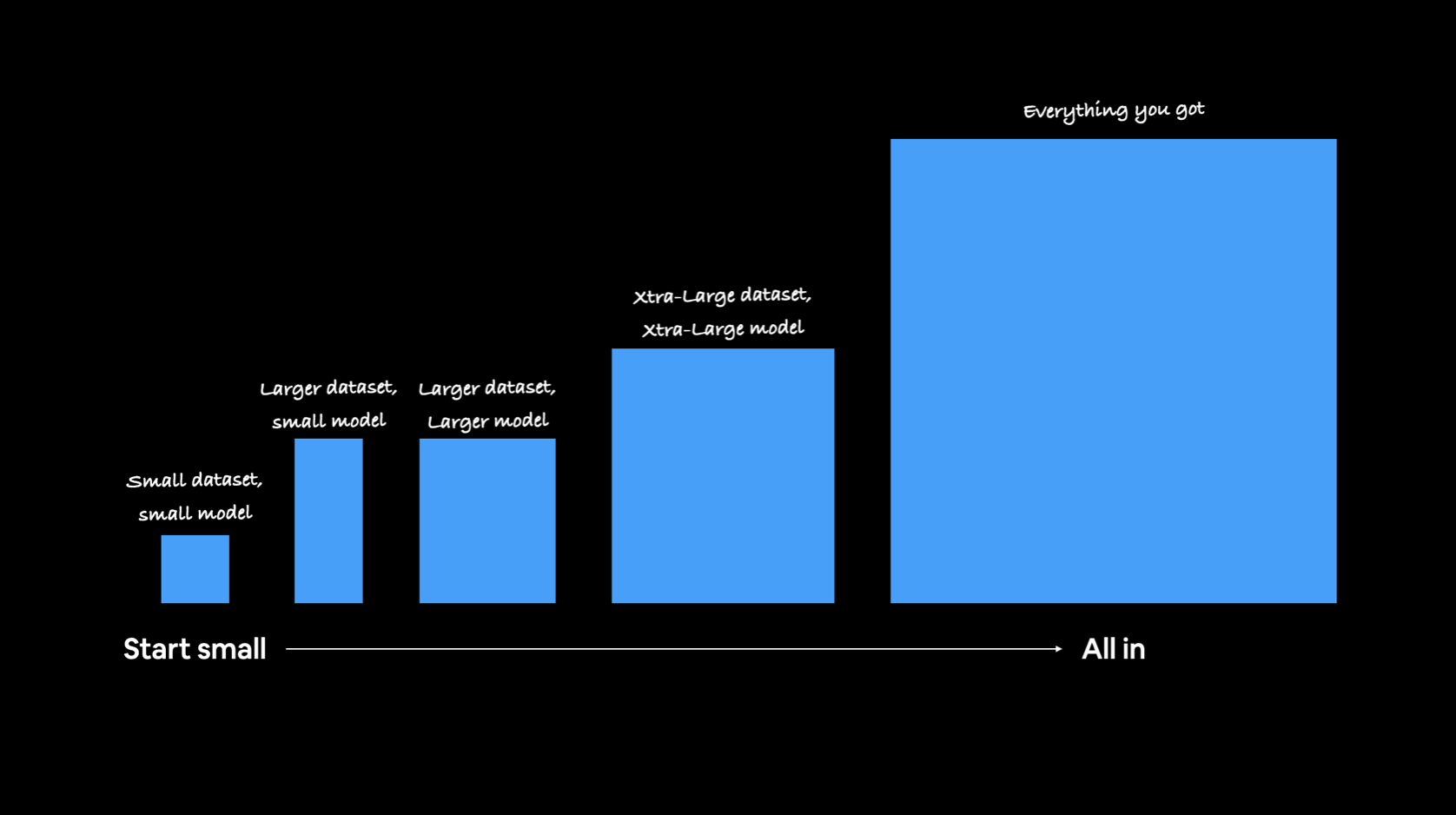 Machine learning practitioners are serial experimenters. Start small, get a model working, see if your experiments work then gradually scale them up to where you want to go (we're going to be looking at scaling up throughout this notebook).
What we're going to cover
We're going to go through the follow with TensorFlow:
- Downloading and preparing 10% of the Food101 data (10% of training data)
- Training a feature extraction transfer learning model on 10% of the Food101 training data
- Fine-tuning our feature extraction model
- Saving and loaded our trained model
- Evaluating the performance of our Food Vision model trained on 10% of the training data
- Finding our model's most wrong predictions
- Making predictions with our Food Vision model on custom images of food
How you can use this notebook
You can read through the descriptions and the code (it should all run, except for the cells which error on purpose), but there's a better option.
Write all of the code yourself.
Yes. I'm serious. Create a new notebook, and rewrite each line by yourself. Investigate it, see if you can break it, why does it break?
You don't have to write the text descriptions but writing the code yourself is a great way to get hands-on experience.
Don't worry if you make mistakes, we all do. The way to get better and make less mistakes is to write more code.
📖 Resources:
- See the full set of course materials on GitHub: https://github.com/mrdbourke/tensorflow-deep-learning
- See updates for this notebook here: https://github.com/mrdbourke/tensorflow-deep-learning/discussions/549
# Are we using a GPU?
# If not, and you're in Google Colab, go to Runtime -> Change runtime type -> Hardware accelerator -> GPU
!nvidia-smi
Thu May 18 02:18:58 2023
+-----------------------------------------------------------------------------+
| NVIDIA-SMI 525.85.12 Driver Version: 525.85.12 CUDA Version: 12.0 |
|-------------------------------+----------------------+----------------------+
| GPU Name Persistence-M| Bus-Id Disp.A | Volatile Uncorr. ECC |
| Fan Temp Perf Pwr:Usage/Cap| Memory-Usage | GPU-Util Compute M. |
| | | MIG M. |
|===============================+======================+======================|
| 0 NVIDIA A100-SXM... Off | 00000000:00:04.0 Off | 0 |
| N/A 45C P0 49W / 400W | 0MiB / 40960MiB | 0% Default |
| | | Disabled |
+-------------------------------+----------------------+----------------------+
+-----------------------------------------------------------------------------+
| Processes: |
| GPU GI CI PID Type Process name GPU Memory |
| ID ID Usage |
|=============================================================================|
| No running processes found |
+-----------------------------------------------------------------------------+
import datetime
print(f"Notebook last run (end-to-end): {datetime.datetime.now()}")
Notebook last run (end-to-end): 2023-05-18 02:18:58.717388
Creating helper functions
We've created a series of helper functions throughout the previous notebooks. Instead of rewriting them (tedious), we'll import the helper_functions.py file from the GitHub repo.
# Get helper functions file
!wget https://raw.githubusercontent.com/mrdbourke/tensorflow-deep-learning/main/extras/helper_functions.py
--2023-05-18 02:18:58-- https://raw.githubusercontent.com/mrdbourke/tensorflow-deep-learning/main/extras/helper_functions.py Resolving raw.githubusercontent.com (raw.githubusercontent.com)... 185.199.108.133, 185.199.109.133, 185.199.110.133, ... Connecting to raw.githubusercontent.com (raw.githubusercontent.com)|185.199.108.133|:443... connected. HTTP request sent, awaiting response... 200 OK Length: 10246 (10K) [text/plain] Saving to: ‘helper_functions.py’ helper_functions.py 0%[ ] 0 --.-KB/s helper_functions.py 100%[===================>] 10.01K --.-KB/s in 0s 2023-05-18 02:18:58 (109 MB/s) - ‘helper_functions.py’ saved [10246/10246]
# Import series of helper functions for the notebook (we've created/used these in previous notebooks)
from helper_functions import create_tensorboard_callback, plot_loss_curves, unzip_data, compare_historys, walk_through_dir
101 Food Classes: Working with less data
So far we've confirmed the transfer learning model's we've been using work pretty well with the 10 Food Classes dataset. Now it's time to step it up and see how they go with the full 101 Food Classes.
In the original Food101 dataset there's 1000 images per class (750 of each class in the training set and 250 of each class in the test set), totalling 101,000 imags.
We could start modelling straight away on this large dataset but in the spirit of continually experimenting, we're going to see how our previously working model's go with 10% of the training data.
This means for each of the 101 food classes we'll be building a model on 75 training images and evaluating it on 250 test images.
Downloading and preprocessing the data
Just as before we'll download a subset of the Food101 dataset which has been extracted from the original dataset (to see the preprocessing of the data check out the Food Vision preprocessing notebook).
We download the data as a zip file so we'll use our unzip_data() function to unzip it.
# Download data from Google Storage (already preformatted)
!wget https://storage.googleapis.com/ztm_tf_course/food_vision/101_food_classes_10_percent.zip
unzip_data("101_food_classes_10_percent.zip")
train_dir = "101_food_classes_10_percent/train/"
test_dir = "101_food_classes_10_percent/test/"
--2023-05-18 02:19:02-- https://storage.googleapis.com/ztm_tf_course/food_vision/101_food_classes_10_percent.zip Resolving storage.googleapis.com (storage.googleapis.com)... 142.250.141.128, 142.251.2.128, 2607:f8b0:4023:c03::80, ... Connecting to storage.googleapis.com (storage.googleapis.com)|142.250.141.128|:443... connected. HTTP request sent, awaiting response... 200 OK Length: 1625420029 (1.5G) [application/zip] Saving to: ‘101_food_classes_10_percent.zip’ 101_food_classes_10 100%[===================>] 1.51G 196MB/s in 7.9s 2023-05-18 02:19:10 (197 MB/s) - ‘101_food_classes_10_percent.zip’ saved [1625420029/1625420029]
# How many images/classes are there?
walk_through_dir("101_food_classes_10_percent")
There are 2 directories and 0 images in '101_food_classes_10_percent'. There are 101 directories and 0 images in '101_food_classes_10_percent/train'. There are 0 directories and 75 images in '101_food_classes_10_percent/train/dumplings'. There are 0 directories and 75 images in '101_food_classes_10_percent/train/ceviche'. There are 0 directories and 75 images in '101_food_classes_10_percent/train/cheese_plate'. There are 0 directories and 75 images in '101_food_classes_10_percent/train/spring_rolls'. There are 0 directories and 75 images in '101_food_classes_10_percent/train/hot_dog'. There are 0 directories and 75 images in '101_food_classes_10_percent/train/tacos'. There are 0 directories and 75 images in '101_food_classes_10_percent/train/cup_cakes'. There are 0 directories and 75 images in '101_food_classes_10_percent/train/samosa'. There are 0 directories and 75 images in '101_food_classes_10_percent/train/gnocchi'. There are 0 directories and 75 images in '101_food_classes_10_percent/train/pad_thai'. There are 0 directories and 75 images in '101_food_classes_10_percent/train/french_fries'. There are 0 directories and 75 images in '101_food_classes_10_percent/train/spaghetti_carbonara'. There are 0 directories and 75 images in '101_food_classes_10_percent/train/huevos_rancheros'. There are 0 directories and 75 images in '101_food_classes_10_percent/train/frozen_yogurt'. There are 0 directories and 75 images in '101_food_classes_10_percent/train/gyoza'. There are 0 directories and 75 images in '101_food_classes_10_percent/train/spaghetti_bolognese'. There are 0 directories and 75 images in '101_food_classes_10_percent/train/eggs_benedict'. There are 0 directories and 75 images in '101_food_classes_10_percent/train/miso_soup'. There are 0 directories and 75 images in '101_food_classes_10_percent/train/hummus'. There are 0 directories and 75 images in '101_food_classes_10_percent/train/lasagna'. There are 0 directories and 75 images in '101_food_classes_10_percent/train/mussels'. There are 0 directories and 75 images in '101_food_classes_10_percent/train/ice_cream'. There are 0 directories and 75 images in '101_food_classes_10_percent/train/foie_gras'. There are 0 directories and 75 images in '101_food_classes_10_percent/train/chocolate_mousse'. There are 0 directories and 75 images in '101_food_classes_10_percent/train/beet_salad'. There are 0 directories and 75 images in '101_food_classes_10_percent/train/poutine'. There are 0 directories and 75 images in '101_food_classes_10_percent/train/garlic_bread'. There are 0 directories and 75 images in '101_food_classes_10_percent/train/waffles'. There are 0 directories and 75 images in '101_food_classes_10_percent/train/peking_duck'. There are 0 directories and 75 images in '101_food_classes_10_percent/train/caprese_salad'. There are 0 directories and 75 images in '101_food_classes_10_percent/train/fried_calamari'. There are 0 directories and 75 images in '101_food_classes_10_percent/train/fish_and_chips'. There are 0 directories and 75 images in '101_food_classes_10_percent/train/macaroni_and_cheese'. There are 0 directories and 75 images in '101_food_classes_10_percent/train/crab_cakes'. There are 0 directories and 75 images in '101_food_classes_10_percent/train/french_onion_soup'. There are 0 directories and 75 images in '101_food_classes_10_percent/train/caesar_salad'. There are 0 directories and 75 images in '101_food_classes_10_percent/train/baklava'. There are 0 directories and 75 images in '101_food_classes_10_percent/train/pizza'. There are 0 directories and 75 images in '101_food_classes_10_percent/train/escargots'. There are 0 directories and 75 images in '101_food_classes_10_percent/train/carrot_cake'. There are 0 directories and 75 images in '101_food_classes_10_percent/train/lobster_bisque'. There are 0 directories and 75 images in '101_food_classes_10_percent/train/beignets'. There are 0 directories and 75 images in '101_food_classes_10_percent/train/apple_pie'. There are 0 directories and 75 images in '101_food_classes_10_percent/train/donuts'. There are 0 directories and 75 images in '101_food_classes_10_percent/train/prime_rib'. There are 0 directories and 75 images in '101_food_classes_10_percent/train/cheesecake'. There are 0 directories and 75 images in '101_food_classes_10_percent/train/scallops'. There are 0 directories and 75 images in '101_food_classes_10_percent/train/bruschetta'. There are 0 directories and 75 images in '101_food_classes_10_percent/train/pulled_pork_sandwich'. There are 0 directories and 75 images in '101_food_classes_10_percent/train/chocolate_cake'. There are 0 directories and 75 images in '101_food_classes_10_percent/train/pork_chop'. There are 0 directories and 75 images in '101_food_classes_10_percent/train/croque_madame'. There are 0 directories and 75 images in '101_food_classes_10_percent/train/sushi'. There are 0 directories and 75 images in '101_food_classes_10_percent/train/paella'. There are 0 directories and 75 images in '101_food_classes_10_percent/train/ramen'. There are 0 directories and 75 images in '101_food_classes_10_percent/train/edamame'. There are 0 directories and 75 images in '101_food_classes_10_percent/train/macarons'. There are 0 directories and 75 images in '101_food_classes_10_percent/train/deviled_eggs'. There are 0 directories and 75 images in '101_food_classes_10_percent/train/oysters'. There are 0 directories and 75 images in '101_food_classes_10_percent/train/chicken_wings'. There are 0 directories and 75 images in '101_food_classes_10_percent/train/hot_and_sour_soup'. There are 0 directories and 75 images in '101_food_classes_10_percent/train/onion_rings'. There are 0 directories and 75 images in '101_food_classes_10_percent/train/churros'. There are 0 directories and 75 images in '101_food_classes_10_percent/train/french_toast'. There are 0 directories and 75 images in '101_food_classes_10_percent/train/risotto'. There are 0 directories and 75 images in '101_food_classes_10_percent/train/chicken_curry'. There are 0 directories and 75 images in '101_food_classes_10_percent/train/club_sandwich'. There are 0 directories and 75 images in '101_food_classes_10_percent/train/chicken_quesadilla'. There are 0 directories and 75 images in '101_food_classes_10_percent/train/hamburger'. There are 0 directories and 75 images in '101_food_classes_10_percent/train/steak'. There are 0 directories and 75 images in '101_food_classes_10_percent/train/beef_carpaccio'. There are 0 directories and 75 images in '101_food_classes_10_percent/train/tuna_tartare'. There are 0 directories and 75 images in '101_food_classes_10_percent/train/greek_salad'. There are 0 directories and 75 images in '101_food_classes_10_percent/train/omelette'. There are 0 directories and 75 images in '101_food_classes_10_percent/train/shrimp_and_grits'. There are 0 directories and 75 images in '101_food_classes_10_percent/train/panna_cotta'. There are 0 directories and 75 images in '101_food_classes_10_percent/train/grilled_cheese_sandwich'. There are 0 directories and 75 images in '101_food_classes_10_percent/train/clam_chowder'. There are 0 directories and 75 images in '101_food_classes_10_percent/train/sashimi'. There are 0 directories and 75 images in '101_food_classes_10_percent/train/cannoli'. There are 0 directories and 75 images in '101_food_classes_10_percent/train/creme_brulee'. There are 0 directories and 75 images in '101_food_classes_10_percent/train/seaweed_salad'. There are 0 directories and 75 images in '101_food_classes_10_percent/train/strawberry_shortcake'. There are 0 directories and 75 images in '101_food_classes_10_percent/train/guacamole'. There are 0 directories and 75 images in '101_food_classes_10_percent/train/breakfast_burrito'. There are 0 directories and 75 images in '101_food_classes_10_percent/train/ravioli'. There are 0 directories and 75 images in '101_food_classes_10_percent/train/pho'. There are 0 directories and 75 images in '101_food_classes_10_percent/train/takoyaki'. There are 0 directories and 75 images in '101_food_classes_10_percent/train/grilled_salmon'. There are 0 directories and 75 images in '101_food_classes_10_percent/train/pancakes'. There are 0 directories and 75 images in '101_food_classes_10_percent/train/falafel'. There are 0 directories and 75 images in '101_food_classes_10_percent/train/filet_mignon'. There are 0 directories and 75 images in '101_food_classes_10_percent/train/beef_tartare'. There are 0 directories and 75 images in '101_food_classes_10_percent/train/lobster_roll_sandwich'. There are 0 directories and 75 images in '101_food_classes_10_percent/train/fried_rice'. There are 0 directories and 75 images in '101_food_classes_10_percent/train/bread_pudding'. There are 0 directories and 75 images in '101_food_classes_10_percent/train/red_velvet_cake'. There are 0 directories and 75 images in '101_food_classes_10_percent/train/nachos'. There are 0 directories and 75 images in '101_food_classes_10_percent/train/tiramisu'. There are 0 directories and 75 images in '101_food_classes_10_percent/train/baby_back_ribs'. There are 0 directories and 75 images in '101_food_classes_10_percent/train/bibimbap'. There are 101 directories and 0 images in '101_food_classes_10_percent/test'. There are 0 directories and 250 images in '101_food_classes_10_percent/test/dumplings'. There are 0 directories and 250 images in '101_food_classes_10_percent/test/ceviche'. There are 0 directories and 250 images in '101_food_classes_10_percent/test/cheese_plate'. There are 0 directories and 250 images in '101_food_classes_10_percent/test/spring_rolls'. There are 0 directories and 250 images in '101_food_classes_10_percent/test/hot_dog'. There are 0 directories and 250 images in '101_food_classes_10_percent/test/tacos'. There are 0 directories and 250 images in '101_food_classes_10_percent/test/cup_cakes'. There are 0 directories and 250 images in '101_food_classes_10_percent/test/samosa'. There are 0 directories and 250 images in '101_food_classes_10_percent/test/gnocchi'. There are 0 directories and 250 images in '101_food_classes_10_percent/test/pad_thai'. There are 0 directories and 250 images in '101_food_classes_10_percent/test/french_fries'. There are 0 directories and 250 images in '101_food_classes_10_percent/test/spaghetti_carbonara'. There are 0 directories and 250 images in '101_food_classes_10_percent/test/huevos_rancheros'. There are 0 directories and 250 images in '101_food_classes_10_percent/test/frozen_yogurt'. There are 0 directories and 250 images in '101_food_classes_10_percent/test/gyoza'. There are 0 directories and 250 images in '101_food_classes_10_percent/test/spaghetti_bolognese'. There are 0 directories and 250 images in '101_food_classes_10_percent/test/eggs_benedict'. There are 0 directories and 250 images in '101_food_classes_10_percent/test/miso_soup'. There are 0 directories and 250 images in '101_food_classes_10_percent/test/hummus'. There are 0 directories and 250 images in '101_food_classes_10_percent/test/lasagna'. There are 0 directories and 250 images in '101_food_classes_10_percent/test/mussels'. There are 0 directories and 250 images in '101_food_classes_10_percent/test/ice_cream'. There are 0 directories and 250 images in '101_food_classes_10_percent/test/foie_gras'. There are 0 directories and 250 images in '101_food_classes_10_percent/test/chocolate_mousse'. There are 0 directories and 250 images in '101_food_classes_10_percent/test/beet_salad'. There are 0 directories and 250 images in '101_food_classes_10_percent/test/poutine'. There are 0 directories and 250 images in '101_food_classes_10_percent/test/garlic_bread'. There are 0 directories and 250 images in '101_food_classes_10_percent/test/waffles'. There are 0 directories and 250 images in '101_food_classes_10_percent/test/peking_duck'. There are 0 directories and 250 images in '101_food_classes_10_percent/test/caprese_salad'. There are 0 directories and 250 images in '101_food_classes_10_percent/test/fried_calamari'. There are 0 directories and 250 images in '101_food_classes_10_percent/test/fish_and_chips'. There are 0 directories and 250 images in '101_food_classes_10_percent/test/macaroni_and_cheese'. There are 0 directories and 250 images in '101_food_classes_10_percent/test/crab_cakes'. There are 0 directories and 250 images in '101_food_classes_10_percent/test/french_onion_soup'. There are 0 directories and 250 images in '101_food_classes_10_percent/test/caesar_salad'. There are 0 directories and 250 images in '101_food_classes_10_percent/test/baklava'. There are 0 directories and 250 images in '101_food_classes_10_percent/test/pizza'. There are 0 directories and 250 images in '101_food_classes_10_percent/test/escargots'. There are 0 directories and 250 images in '101_food_classes_10_percent/test/carrot_cake'. There are 0 directories and 250 images in '101_food_classes_10_percent/test/lobster_bisque'. There are 0 directories and 250 images in '101_food_classes_10_percent/test/beignets'. There are 0 directories and 250 images in '101_food_classes_10_percent/test/apple_pie'. There are 0 directories and 250 images in '101_food_classes_10_percent/test/donuts'. There are 0 directories and 250 images in '101_food_classes_10_percent/test/prime_rib'. There are 0 directories and 250 images in '101_food_classes_10_percent/test/cheesecake'. There are 0 directories and 250 images in '101_food_classes_10_percent/test/scallops'. There are 0 directories and 250 images in '101_food_classes_10_percent/test/bruschetta'. There are 0 directories and 250 images in '101_food_classes_10_percent/test/pulled_pork_sandwich'. There are 0 directories and 250 images in '101_food_classes_10_percent/test/chocolate_cake'. There are 0 directories and 250 images in '101_food_classes_10_percent/test/pork_chop'. There are 0 directories and 250 images in '101_food_classes_10_percent/test/croque_madame'. There are 0 directories and 250 images in '101_food_classes_10_percent/test/sushi'. There are 0 directories and 250 images in '101_food_classes_10_percent/test/paella'. There are 0 directories and 250 images in '101_food_classes_10_percent/test/ramen'. There are 0 directories and 250 images in '101_food_classes_10_percent/test/edamame'. There are 0 directories and 250 images in '101_food_classes_10_percent/test/macarons'. There are 0 directories and 250 images in '101_food_classes_10_percent/test/deviled_eggs'. There are 0 directories and 250 images in '101_food_classes_10_percent/test/oysters'. There are 0 directories and 250 images in '101_food_classes_10_percent/test/chicken_wings'. There are 0 directories and 250 images in '101_food_classes_10_percent/test/hot_and_sour_soup'. There are 0 directories and 250 images in '101_food_classes_10_percent/test/onion_rings'. There are 0 directories and 250 images in '101_food_classes_10_percent/test/churros'. There are 0 directories and 250 images in '101_food_classes_10_percent/test/french_toast'. There are 0 directories and 250 images in '101_food_classes_10_percent/test/risotto'. There are 0 directories and 250 images in '101_food_classes_10_percent/test/chicken_curry'. There are 0 directories and 250 images in '101_food_classes_10_percent/test/club_sandwich'. There are 0 directories and 250 images in '101_food_classes_10_percent/test/chicken_quesadilla'. There are 0 directories and 250 images in '101_food_classes_10_percent/test/hamburger'. There are 0 directories and 250 images in '101_food_classes_10_percent/test/steak'. There are 0 directories and 250 images in '101_food_classes_10_percent/test/beef_carpaccio'. There are 0 directories and 250 images in '101_food_classes_10_percent/test/tuna_tartare'. There are 0 directories and 250 images in '101_food_classes_10_percent/test/greek_salad'. There are 0 directories and 250 images in '101_food_classes_10_percent/test/omelette'. There are 0 directories and 250 images in '101_food_classes_10_percent/test/shrimp_and_grits'. There are 0 directories and 250 images in '101_food_classes_10_percent/test/panna_cotta'. There are 0 directories and 250 images in '101_food_classes_10_percent/test/grilled_cheese_sandwich'. There are 0 directories and 250 images in '101_food_classes_10_percent/test/clam_chowder'. There are 0 directories and 250 images in '101_food_classes_10_percent/test/sashimi'. There are 0 directories and 250 images in '101_food_classes_10_percent/test/cannoli'. There are 0 directories and 250 images in '101_food_classes_10_percent/test/creme_brulee'. There are 0 directories and 250 images in '101_food_classes_10_percent/test/seaweed_salad'. There are 0 directories and 250 images in '101_food_classes_10_percent/test/strawberry_shortcake'. There are 0 directories and 250 images in '101_food_classes_10_percent/test/guacamole'. There are 0 directories and 250 images in '101_food_classes_10_percent/test/breakfast_burrito'. There are 0 directories and 250 images in '101_food_classes_10_percent/test/ravioli'. There are 0 directories and 250 images in '101_food_classes_10_percent/test/pho'. There are 0 directories and 250 images in '101_food_classes_10_percent/test/takoyaki'. There are 0 directories and 250 images in '101_food_classes_10_percent/test/grilled_salmon'. There are 0 directories and 250 images in '101_food_classes_10_percent/test/pancakes'. There are 0 directories and 250 images in '101_food_classes_10_percent/test/falafel'. There are 0 directories and 250 images in '101_food_classes_10_percent/test/filet_mignon'. There are 0 directories and 250 images in '101_food_classes_10_percent/test/beef_tartare'. There are 0 directories and 250 images in '101_food_classes_10_percent/test/lobster_roll_sandwich'. There are 0 directories and 250 images in '101_food_classes_10_percent/test/fried_rice'. There are 0 directories and 250 images in '101_food_classes_10_percent/test/bread_pudding'. There are 0 directories and 250 images in '101_food_classes_10_percent/test/red_velvet_cake'. There are 0 directories and 250 images in '101_food_classes_10_percent/test/nachos'. There are 0 directories and 250 images in '101_food_classes_10_percent/test/tiramisu'. There are 0 directories and 250 images in '101_food_classes_10_percent/test/baby_back_ribs'. There are 0 directories and 250 images in '101_food_classes_10_percent/test/bibimbap'.
As before our data comes in the common image classification data format of:
Example of file structure
10_food_classes_10_percent <- top level folder
└───train <- training images
│ └───pizza
│ │ │ 1008104.jpg
│ │ │ 1638227.jpg
│ │ │ ...
│ └───steak
│ │ 1000205.jpg
│ │ 1647351.jpg
│ │ ...
│
└───test <- testing images
│ └───pizza
│ │ │ 1001116.jpg
│ │ │ 1507019.jpg
│ │ │ ...
│ └───steak
│ │ 100274.jpg
│ │ 1653815.jpg
│ │ ...
Let's use the image_dataset_from_directory() function to turn our images and labels into a tf.data.Dataset, a TensorFlow datatype which allows for us to pass it directory to our model.
For the test dataset, we're going to set shuffle=False so we can perform repeatable evaluation and visualization on it later.
# Setup data inputs
import tensorflow as tf
IMG_SIZE = (224, 224)
train_data_all_10_percent = tf.keras.preprocessing.image_dataset_from_directory(train_dir,
label_mode="categorical",
image_size=IMG_SIZE)
test_data = tf.keras.preprocessing.image_dataset_from_directory(test_dir,
label_mode="categorical",
image_size=IMG_SIZE,
shuffle=False) # don't shuffle test data for prediction analysis
Found 7575 files belonging to 101 classes. Found 25250 files belonging to 101 classes.
Wonderful! It looks like our data has been imported as expected with 75 images per class in the training set (75 images * 101 classes = 7575 images) and 25250 images in the test set (250 images * 101 classes = 25250 images).
Train a big dog model with transfer learning on 10% of 101 food classes
Our food image data has been imported into TensorFlow, time to model it.
To keep our experiments swift, we're going to start by using feature extraction transfer learning with a pre-trained model for a few epochs and then fine-tune for a few more epochs.
More specifically, our goal will be to see if we can beat the baseline from original Food101 paper (50.76% accuracy on 101 classes) with 10% of the training data and the following modelling setup:
- A
ModelCheckpointcallback to save our progress during training, this means we could experiment with further training later without having to train from scratch every time - Data augmentation built right into the model
- A headless (no top layers)
EfficientNetB0architecture fromtf.keras.applicationsas our base model - A
Denselayer with 101 hidden neurons (same as number of food classes) and softmax activation as the output layer - Categorical crossentropy as the loss function since we're dealing with more than two classes
- The Adam optimizer with the default settings
- Fitting for 5 full passes on the training data while evaluating on 15% of the test data
It seems like a lot but these are all things we've covered before in the Transfer Learning in TensorFlow Part 2: Fine-tuning notebook.
Let's start by creating the ModelCheckpoint callback.
Since we want our model to perform well on unseen data we'll set it to monitor the validation accuracy metric and save the model weights which score the best on that.
# Create checkpoint callback to save model for later use
checkpoint_path = "101_classes_10_percent_data_model_checkpoint"
checkpoint_callback = tf.keras.callbacks.ModelCheckpoint(checkpoint_path,
save_weights_only=True, # save only the model weights
monitor="val_accuracy", # save the model weights which score the best validation accuracy
save_best_only=True) # only keep the best model weights on file (delete the rest)
Checkpoint ready. Now let's create a small data augmentation model with the Sequential API. Because we're working with a reduced sized training set, this will help prevent our model from overfitting on the training data.
# Import the required modules for model creation
from tensorflow.keras import layers
from tensorflow.keras.models import Sequential
## NEW: Newer versions of TensorFlow (2.10+) can use the tensorflow.keras.layers API directly for data augmentation
data_augmentation = Sequential([
layers.RandomFlip("horizontal"),
layers.RandomRotation(0.2),
layers.RandomZoom(0.2),
layers.RandomHeight(0.2),
layers.RandomWidth(0.2),
# preprocessing.Rescaling(1./255) # keep for ResNet50V2, remove for EfficientNetB0
], name ="data_augmentation")
## OLD
# # Setup data augmentation
# from tensorflow.keras.layers.experimental import preprocessing
# data_augmentation = Sequential([
# preprocessing.RandomFlip("horizontal"), # randomly flip images on horizontal edge
# preprocessing.RandomRotation(0.2), # randomly rotate images by a specific amount
# preprocessing.RandomHeight(0.2), # randomly adjust the height of an image by a specific amount
# preprocessing.RandomWidth(0.2), # randomly adjust the width of an image by a specific amount
# preprocessing.RandomZoom(0.2), # randomly zoom into an image
# # preprocessing.Rescaling(1./255) # keep for models like ResNet50V2, remove for EfficientNet
# ], name="data_augmentation")
Beautiful! We'll be able to insert the data_augmentation Sequential model as a layer in our Functional API model. That way if we want to continue training our model at a later time, the data augmentation is already built right in.
Speaking of Functional API model's, time to put together a feature extraction transfer learning model using tf.keras.applications.efficientnet.EfficientNetB0 as our base model.
We'll import the base model using the parameter include_top=False so we can add on our own output layers, notably GlobalAveragePooling2D() (condense the outputs of the base model into a shape usable by the output layer) followed by a Dense layer.
# Setup base model and freeze its layers (this will extract features)
base_model = tf.keras.applications.efficientnet.EfficientNetB0(include_top=False)
base_model.trainable = False
# Setup model architecture with trainable top layers
inputs = layers.Input(shape=(224, 224, 3), name="input_layer") # shape of input image
x = data_augmentation(inputs) # augment images (only happens during training)
x = base_model(x, training=False) # put the base model in inference mode so we can use it to extract features without updating the weights
x = layers.GlobalAveragePooling2D(name="global_average_pooling")(x) # pool the outputs of the base model
outputs = layers.Dense(len(train_data_all_10_percent.class_names), activation="softmax", name="output_layer")(x) # same number of outputs as classes
model = tf.keras.Model(inputs, outputs)
Downloading data from https://storage.googleapis.com/keras-applications/efficientnetb0_notop.h5 16705208/16705208 [==============================] - 0s 0us/step
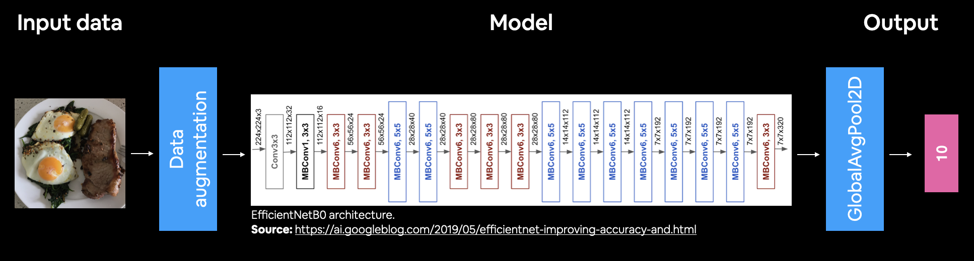 A colourful figure of the model we've created with: 224x224 images as input, data augmentation as a layer, EfficientNetB0 as a backbone, an averaging pooling layer as well as dense layer with 10 neurons (same as number of classes we're working with) as output.
Model created. Let's inspect it.
# Get a summary of our model
model.summary()
Model: "model"
_________________________________________________________________
Layer (type) Output Shape Param #
=================================================================
input_layer (InputLayer) [(None, 224, 224, 3)] 0
data_augmentation (Sequenti (None, None, None, 3) 0
al)
efficientnetb0 (Functional) (None, None, None, 1280) 4049571
global_average_pooling (Glo (None, 1280) 0
balAveragePooling2D)
output_layer (Dense) (None, 101) 129381
=================================================================
Total params: 4,178,952
Trainable params: 129,381
Non-trainable params: 4,049,571
_________________________________________________________________
Looking good! Our Functional model has 5 layers but each of those layers have varying amounts of layers within them.
Notice the number of trainable and non-trainable parameters. It seems the only trainable parameters are within the output_layer which is exactly what we're after with this first run of feature extraction; keep all the learned patterns in the base model (EfficientNetb0) frozen whilst allowing the model to tune its outputs to our custom data.
Time to compile and fit.
# Compile
model.compile(loss="categorical_crossentropy",
optimizer=tf.keras.optimizers.Adam(), # use Adam with default settings
metrics=["accuracy"])
# Fit
history_all_classes_10_percent = model.fit(train_data_all_10_percent,
epochs=5, # fit for 5 epochs to keep experiments quick
validation_data=test_data,
validation_steps=int(0.15 * len(test_data)), # evaluate on smaller portion of test data
callbacks=[checkpoint_callback]) # save best model weights to file
Epoch 1/5 237/237 [==============================] - 29s 59ms/step - loss: 3.3881 - accuracy: 0.2796 - val_loss: 2.4697 - val_accuracy: 0.4661 Epoch 2/5 237/237 [==============================] - 12s 51ms/step - loss: 2.1996 - accuracy: 0.4937 - val_loss: 2.0252 - val_accuracy: 0.5188 Epoch 3/5 237/237 [==============================] - 12s 51ms/step - loss: 1.8245 - accuracy: 0.5675 - val_loss: 1.8783 - val_accuracy: 0.5344 Epoch 4/5 237/237 [==============================] - 12s 50ms/step - loss: 1.6061 - accuracy: 0.6055 - val_loss: 1.8206 - val_accuracy: 0.5355 Epoch 5/5 237/237 [==============================] - 11s 48ms/step - loss: 1.4493 - accuracy: 0.6440 - val_loss: 1.7824 - val_accuracy: 0.5310
Woah! It looks like our model is getting some impressive results, but remember, during training our model only evaluated on 15% of the test data. Let's see how it did on the whole test dataset.
# Evaluate model
results_feature_extraction_model = model.evaluate(test_data)
results_feature_extraction_model
790/790 [==============================] - 16s 21ms/step - loss: 1.5888 - accuracy: 0.5797
[1.5887829065322876, 0.5797227621078491]
Well it looks like we just beat our baseline (the results from the original Food101 paper) with 10% of the data! In under 5-minutes... that's the power of deep learning and more precisely, transfer learning: leveraging what one model has learned on another dataset for our own dataset.
How do the loss curves look?
plot_loss_curves(history_all_classes_10_percent)


🤔 Question: What do these curves suggest? Hint: ideally, the two curves should be very similar to each other, if not, there may be some overfitting or underfitting.
Fine-tuning
Our feature extraction transfer learning model is performing well. Why don't we try to fine-tune a few layers in the base model and see if we gain any improvements?
The good news is, thanks to the ModelCheckpoint callback, we've got the saved weights of our already well-performing model so if fine-tuning doesn't add any benefits, we can revert back.
To fine-tune the base model we'll first set its trainable attribute to True, unfreezing all of the frozen.
Then since we've got a relatively small training dataset, we'll refreeze every layer except for the last 5, making them trainable.
# Unfreeze all of the layers in the base model
base_model.trainable = True
# Refreeze every layer except for the last 5
for layer in base_model.layers[:-5]:
layer.trainable = False
We just made a change to the layers in our model and what do we have to do every time we make a change to our model?
Recompile it.
Because we're fine-tuning, we'll use a 10x lower learning rate to ensure the updates to the previous trained weights aren't too large.
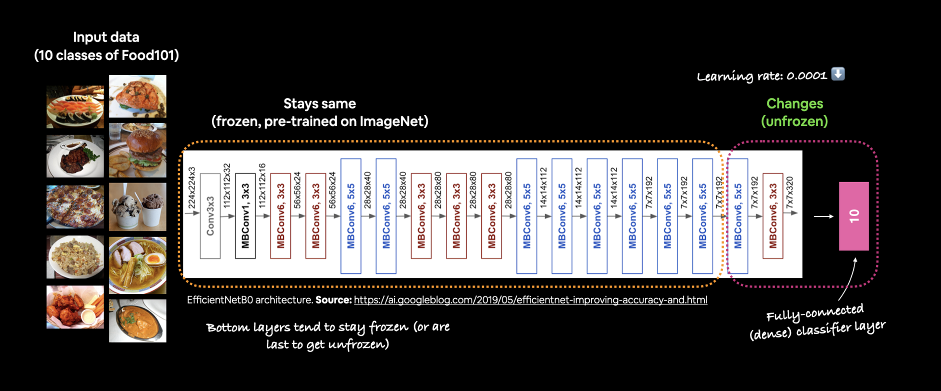 When fine-tuning and unfreezing layers of your pre-trained model, it's common practice to lower the learning rate you used for your feature extraction model. How much by? A 10x lower learning rate is usually a good place to to start.
# Recompile model with lower learning rate
model.compile(loss='categorical_crossentropy',
optimizer=tf.keras.optimizers.Adam(1e-4), # 10x lower learning rate than default
metrics=['accuracy'])
Model recompiled, how about we make sure the layers we want are trainable?
# What layers in the model are trainable?
for layer in model.layers:
print(layer.name, layer.trainable)
input_layer True data_augmentation True efficientnetb0 True global_average_pooling True output_layer True
# Check which layers are trainable
for layer_number, layer in enumerate(base_model.layers):
print(layer_number, layer.name, layer.trainable)
0 input_1 False 1 rescaling False 2 normalization False 3 rescaling_1 False 4 stem_conv_pad False 5 stem_conv False 6 stem_bn False 7 stem_activation False 8 block1a_dwconv False 9 block1a_bn False 10 block1a_activation False 11 block1a_se_squeeze False 12 block1a_se_reshape False 13 block1a_se_reduce False 14 block1a_se_expand False 15 block1a_se_excite False 16 block1a_project_conv False 17 block1a_project_bn False 18 block2a_expand_conv False 19 block2a_expand_bn False 20 block2a_expand_activation False 21 block2a_dwconv_pad False 22 block2a_dwconv False 23 block2a_bn False 24 block2a_activation False 25 block2a_se_squeeze False 26 block2a_se_reshape False 27 block2a_se_reduce False 28 block2a_se_expand False 29 block2a_se_excite False 30 block2a_project_conv False 31 block2a_project_bn False 32 block2b_expand_conv False 33 block2b_expand_bn False 34 block2b_expand_activation False 35 block2b_dwconv False 36 block2b_bn False 37 block2b_activation False 38 block2b_se_squeeze False 39 block2b_se_reshape False 40 block2b_se_reduce False 41 block2b_se_expand False 42 block2b_se_excite False 43 block2b_project_conv False 44 block2b_project_bn False 45 block2b_drop False 46 block2b_add False 47 block3a_expand_conv False 48 block3a_expand_bn False 49 block3a_expand_activation False 50 block3a_dwconv_pad False 51 block3a_dwconv False 52 block3a_bn False 53 block3a_activation False 54 block3a_se_squeeze False 55 block3a_se_reshape False 56 block3a_se_reduce False 57 block3a_se_expand False 58 block3a_se_excite False 59 block3a_project_conv False 60 block3a_project_bn False 61 block3b_expand_conv False 62 block3b_expand_bn False 63 block3b_expand_activation False 64 block3b_dwconv False 65 block3b_bn False 66 block3b_activation False 67 block3b_se_squeeze False 68 block3b_se_reshape False 69 block3b_se_reduce False 70 block3b_se_expand False 71 block3b_se_excite False 72 block3b_project_conv False 73 block3b_project_bn False 74 block3b_drop False 75 block3b_add False 76 block4a_expand_conv False 77 block4a_expand_bn False 78 block4a_expand_activation False 79 block4a_dwconv_pad False 80 block4a_dwconv False 81 block4a_bn False 82 block4a_activation False 83 block4a_se_squeeze False 84 block4a_se_reshape False 85 block4a_se_reduce False 86 block4a_se_expand False 87 block4a_se_excite False 88 block4a_project_conv False 89 block4a_project_bn False 90 block4b_expand_conv False 91 block4b_expand_bn False 92 block4b_expand_activation False 93 block4b_dwconv False 94 block4b_bn False 95 block4b_activation False 96 block4b_se_squeeze False 97 block4b_se_reshape False 98 block4b_se_reduce False 99 block4b_se_expand False 100 block4b_se_excite False 101 block4b_project_conv False 102 block4b_project_bn False 103 block4b_drop False 104 block4b_add False 105 block4c_expand_conv False 106 block4c_expand_bn False 107 block4c_expand_activation False 108 block4c_dwconv False 109 block4c_bn False 110 block4c_activation False 111 block4c_se_squeeze False 112 block4c_se_reshape False 113 block4c_se_reduce False 114 block4c_se_expand False 115 block4c_se_excite False 116 block4c_project_conv False 117 block4c_project_bn False 118 block4c_drop False 119 block4c_add False 120 block5a_expand_conv False 121 block5a_expand_bn False 122 block5a_expand_activation False 123 block5a_dwconv False 124 block5a_bn False 125 block5a_activation False 126 block5a_se_squeeze False 127 block5a_se_reshape False 128 block5a_se_reduce False 129 block5a_se_expand False 130 block5a_se_excite False 131 block5a_project_conv False 132 block5a_project_bn False 133 block5b_expand_conv False 134 block5b_expand_bn False 135 block5b_expand_activation False 136 block5b_dwconv False 137 block5b_bn False 138 block5b_activation False 139 block5b_se_squeeze False 140 block5b_se_reshape False 141 block5b_se_reduce False 142 block5b_se_expand False 143 block5b_se_excite False 144 block5b_project_conv False 145 block5b_project_bn False 146 block5b_drop False 147 block5b_add False 148 block5c_expand_conv False 149 block5c_expand_bn False 150 block5c_expand_activation False 151 block5c_dwconv False 152 block5c_bn False 153 block5c_activation False 154 block5c_se_squeeze False 155 block5c_se_reshape False 156 block5c_se_reduce False 157 block5c_se_expand False 158 block5c_se_excite False 159 block5c_project_conv False 160 block5c_project_bn False 161 block5c_drop False 162 block5c_add False 163 block6a_expand_conv False 164 block6a_expand_bn False 165 block6a_expand_activation False 166 block6a_dwconv_pad False 167 block6a_dwconv False 168 block6a_bn False 169 block6a_activation False 170 block6a_se_squeeze False 171 block6a_se_reshape False 172 block6a_se_reduce False 173 block6a_se_expand False 174 block6a_se_excite False 175 block6a_project_conv False 176 block6a_project_bn False 177 block6b_expand_conv False 178 block6b_expand_bn False 179 block6b_expand_activation False 180 block6b_dwconv False 181 block6b_bn False 182 block6b_activation False 183 block6b_se_squeeze False 184 block6b_se_reshape False 185 block6b_se_reduce False 186 block6b_se_expand False 187 block6b_se_excite False 188 block6b_project_conv False 189 block6b_project_bn False 190 block6b_drop False 191 block6b_add False 192 block6c_expand_conv False 193 block6c_expand_bn False 194 block6c_expand_activation False 195 block6c_dwconv False 196 block6c_bn False 197 block6c_activation False 198 block6c_se_squeeze False 199 block6c_se_reshape False 200 block6c_se_reduce False 201 block6c_se_expand False 202 block6c_se_excite False 203 block6c_project_conv False 204 block6c_project_bn False 205 block6c_drop False 206 block6c_add False 207 block6d_expand_conv False 208 block6d_expand_bn False 209 block6d_expand_activation False 210 block6d_dwconv False 211 block6d_bn False 212 block6d_activation False 213 block6d_se_squeeze False 214 block6d_se_reshape False 215 block6d_se_reduce False 216 block6d_se_expand False 217 block6d_se_excite False 218 block6d_project_conv False 219 block6d_project_bn False 220 block6d_drop False 221 block6d_add False 222 block7a_expand_conv False 223 block7a_expand_bn False 224 block7a_expand_activation False 225 block7a_dwconv False 226 block7a_bn False 227 block7a_activation False 228 block7a_se_squeeze False 229 block7a_se_reshape False 230 block7a_se_reduce False 231 block7a_se_expand False 232 block7a_se_excite False 233 block7a_project_conv True 234 block7a_project_bn True 235 top_conv True 236 top_bn True 237 top_activation True
Excellent! Time to fine-tune our model.
Another 5 epochs should be enough to see whether any benefits come about (though we could always try more).
We'll start the training off where the feature extraction model left off using the initial_epoch parameter in the fit() function.
# Fine-tune for 5 more epochs
fine_tune_epochs = 10 # model has already done 5 epochs, this is the total number of epochs we're after (5+5=10)
history_all_classes_10_percent_fine_tune = model.fit(train_data_all_10_percent,
epochs=fine_tune_epochs,
validation_data=test_data,
validation_steps=int(0.15 * len(test_data)), # validate on 15% of the test data
initial_epoch=history_all_classes_10_percent.epoch[-1]) # start from previous last epoch
Epoch 5/10 237/237 [==============================] - 51s 173ms/step - loss: 1.2195 - accuracy: 0.6764 - val_loss: 1.7268 - val_accuracy: 0.5392 Epoch 6/10 237/237 [==============================] - 25s 104ms/step - loss: 1.1019 - accuracy: 0.7006 - val_loss: 1.7007 - val_accuracy: 0.5493 Epoch 7/10 237/237 [==============================] - 22s 91ms/step - loss: 1.0089 - accuracy: 0.7291 - val_loss: 1.7452 - val_accuracy: 0.5426 Epoch 8/10 237/237 [==============================] - 20s 84ms/step - loss: 0.9453 - accuracy: 0.7480 - val_loss: 1.7133 - val_accuracy: 0.5506 Epoch 9/10 237/237 [==============================] - 19s 79ms/step - loss: 0.8790 - accuracy: 0.7673 - val_loss: 1.7370 - val_accuracy: 0.5471 Epoch 10/10 237/237 [==============================] - 17s 72ms/step - loss: 0.8351 - accuracy: 0.7768 - val_loss: 1.7431 - val_accuracy: 0.5498
Once again, during training we were only evaluating on a small portion of the test data, let's find out how our model went on all of the test data.
# Evaluate fine-tuned model on the whole test dataset
results_all_classes_10_percent_fine_tune = model.evaluate(test_data)
results_all_classes_10_percent_fine_tune
790/790 [==============================] - 16s 21ms/step - loss: 1.5078 - accuracy: 0.6011
[1.5077574253082275, 0.6010693311691284]
Hmm... it seems like our model got a slight boost from fine-tuning.
We might get a better picture by using our compare_historys() function and seeing what the training curves say.
compare_historys(original_history=history_all_classes_10_percent,
new_history=history_all_classes_10_percent_fine_tune,
initial_epochs=5)

It seems that after fine-tuning, our model's training metrics improved significantly but validation, not so much. Looks like our model is starting to overfit.
This is okay though, its very often the case that fine-tuning leads to overfitting when the data a pre-trained model has been trained on is similar to your custom data.
In our case, our pre-trained model, EfficientNetB0 was trained on ImageNet which contains many real life pictures of food just like our food dataset.
If feautre extraction already works well, the improvements you see from fine-tuning may not be as great as if your dataset was significantly different from the data your base model was pre-trained on.
# # Save model to drive so it can be used later
# model.save("drive/My Drive/tensorflow_course/101_food_class_10_percent_saved_big_dog_model")
Evaluating the performance of the big dog model across all different classes
We've got a trained and saved model which according to the evaluation metrics we've used is performing fairly well.
But metrics schmetrics, let's dive a little deeper into our model's performance and get some visualizations going.
To do so, we'll load in the saved model and use it to make some predictions on the test dataset.
🔑 Note: Evaluating a machine learning model is as important as training one. Metrics can be deceiving. You should always visualize your model's performance on unseen data to make sure you aren't being fooled good looking training numbers.
import tensorflow as tf
# Download pre-trained model from Google Storage (like a cooking show, I trained this model earlier, so the results may be different than above)
!wget https://storage.googleapis.com/ztm_tf_course/food_vision/06_101_food_class_10_percent_saved_big_dog_model.zip
saved_model_path = "06_101_food_class_10_percent_saved_big_dog_model.zip"
unzip_data(saved_model_path)
# Note: loading a model will output a lot of 'WARNINGS', these can be ignored: https://www.tensorflow.org/tutorials/keras/save_and_load#save_checkpoints_during_training
# There's also a thread on GitHub trying to fix these warnings: https://github.com/tensorflow/tensorflow/issues/40166
# model = tf.keras.models.load_model("drive/My Drive/tensorflow_course/101_food_class_10_percent_saved_big_dog_model/") # path to drive model
model = tf.keras.models.load_model(saved_model_path.split(".")[0]) # don't include ".zip" in loaded model path
To make sure our loaded model is indead a trained model, let's evaluate its performance on the test dataset.
# Check to see if loaded model is a trained model
loaded_loss, loaded_accuracy = model.evaluate(test_data)
loaded_loss, loaded_accuracy
790/790 [==============================] - 19s 22ms/step - loss: 1.8022 - accuracy: 0.6078
(1.8021684885025024, 0.6078019738197327)
Wonderful! It looks like our loaded model is performing just as well as it was before we saved it. Let's make some predictions.
Making predictions with our trained model
To evaluate our trained model, we need to make some predictions with it and then compare those predictions to the test dataset.
Because the model has never seen the test dataset, this should give us an indication of how the model will perform in the real world on data similar to what it has been trained on.
To make predictions with our trained model, we can use the predict() method passing it the test data.
Since our data is multi-class, doing this will return a prediction probably tensor for each sample.
In other words, every time the trained model see's an image it will compare it to all of the patterns it learned during training and return an output for every class (all 101 of them) of how likely the image is to be that class.
# Make predictions with model
pred_probs = model.predict(test_data, verbose=1) # set verbosity to see how long it will take
790/790 [==============================] - 15s 18ms/step
We just passed all of the test images to our model and asked it to make a prediction on what food it thinks is in each.
So if we had 25250 images in the test dataset, how many predictions do you think we should have?
# How many predictions are there?
len(pred_probs)
25250
And if each image could be one of 101 classes, how many predictions do you think we'll have for each image?
# What's the shape of our predictions?
pred_probs.shape
(25250, 101)
What we've got is often referred to as a predictions probability tensor (or array).
Let's see what the first 10 look like.
# How do they look?
pred_probs[:10]
array([[5.9555572e-02, 3.5662119e-06, 4.1279349e-02, ..., 1.4194699e-09,
8.4039129e-05, 3.0820314e-03],
[9.6338320e-01, 1.3765826e-09, 8.5042708e-04, ..., 5.4804143e-05,
7.8341188e-12, 9.7811304e-10],
[9.5942634e-01, 3.2432759e-05, 1.4769287e-03, ..., 7.1438910e-07,
5.5323352e-07, 4.0179562e-05],
...,
[4.7279873e-01, 1.2954312e-07, 1.4748254e-03, ..., 5.9630687e-04,
6.7163957e-05, 2.3532135e-05],
[4.4502247e-02, 4.7261000e-07, 1.2174438e-01, ..., 6.2917384e-06,
7.5576504e-06, 3.6633476e-03],
[7.2373080e-01, 1.9256416e-09, 5.2089705e-05, ..., 1.2218992e-03,
1.5755526e-09, 9.6206924e-05]], dtype=float32)
Alright, it seems like we've got a bunch of tensors of really small numbers, how about we zoom into one of them?
# We get one prediction probability per class
print(f"Number of prediction probabilities for sample 0: {len(pred_probs[0])}")
print(f"What prediction probability sample 0 looks like:\n {pred_probs[0]}")
print(f"The class with the highest predicted probability by the model for sample 0: {pred_probs[0].argmax()}")
Number of prediction probabilities for sample 0: 101 What prediction probability sample 0 looks like: [5.95555715e-02 3.56621194e-06 4.12793495e-02 1.06392506e-09 8.19964274e-09 8.61560245e-09 8.10409119e-07 8.49006710e-07 1.98095986e-05 7.99297993e-07 3.17695403e-09 9.83702989e-07 2.83578265e-04 7.78589082e-10 7.43659853e-04 3.87942600e-05 6.44463080e-06 2.50333073e-06 3.77276956e-05 2.05599179e-07 1.55429479e-05 8.10427650e-07 2.60885736e-06 2.03088433e-07 8.30327224e-07 5.42988437e-06 3.74273668e-06 1.32360203e-08 2.74555851e-03 2.79426695e-05 6.86718571e-10 2.53517483e-05 1.66382728e-04 7.57455043e-10 4.02367179e-04 1.30578828e-08 1.79280721e-06 1.43956686e-06 2.30789818e-02 8.24019480e-07 8.61712351e-07 1.69789450e-06 7.03542946e-06 1.85722051e-08 2.87577478e-07 7.99586633e-06 2.07466110e-06 1.86462174e-07 3.34909487e-08 3.17168073e-04 1.04948031e-05 8.55388123e-07 8.47566068e-01 1.05432355e-05 4.34703423e-07 3.72825380e-05 3.50601949e-05 3.25856490e-05 6.74493349e-05 1.27383810e-08 2.62344230e-10 1.03191360e-05 8.54040845e-05 1.05053311e-06 2.11897259e-06 3.72938448e-05 7.52453388e-08 2.50746176e-04 9.31413410e-07 1.24124577e-04 6.20197443e-06 1.24211716e-08 4.04207458e-05 6.82277772e-08 1.24867688e-06 5.15563556e-08 7.48909628e-08 7.54529829e-05 7.75354492e-05 6.31509749e-07 9.79340939e-07 2.18733803e-05 1.49467369e-05 1.39609512e-07 1.22257961e-05 1.90126449e-02 4.97255787e-05 4.59980038e-06 1.51860661e-07 3.38210441e-07 3.89491328e-09 1.64673807e-07 8.08345867e-05 4.90067578e-06 2.41164742e-07 2.32299317e-05 3.09399824e-04 3.10968826e-05 1.41946987e-09 8.40391294e-05 3.08203138e-03] The class with the highest predicted probability by the model for sample 0: 52
As we discussed before, for each image tensor we pass to our model, because of the number of output neurons and activation function in the last layer (layers.Dense(len(train_data_all_10_percent.class_names), activation="softmax"), it outputs a prediction probability between 0 and 1 for all each of the 101 classes.
And the index of the highest prediction probability can be considered what the model thinks is the most likely label. Similarly, the lower prediction probaiblity value, the less the model thinks that the target image is that specific class.
🔑 Note: Due to the nature of the softmax activation function, the sum of each of the prediction probabilities for a single sample will be 1 (or at least very close to 1). E.g.
pred_probs[0].sum() = 1.
We can find the index of the maximum value in each prediction probability tensor using the argmax() method.
# Get the class predicitons of each label
pred_classes = pred_probs.argmax(axis=1)
# How do they look?
pred_classes[:10]
array([52, 0, 0, 80, 79, 61, 29, 0, 85, 0])
Beautiful! We've now got the predicted class index for each of the samples in our test dataset.
We'll be able to compare these to the test dataset labels to further evaluate our model.
To get the test dataset labels we can unravel our test_data object (which is in the form of a tf.data.Dataset) using the unbatch() method.
Doing this will give us access to the images and labels in the test dataset. Since the labels are in one-hot encoded format, we'll take use the argmax() method to return the index of the label.
🔑 Note: This unravelling is why we
shuffle=Falsewhen creating the test data object. Otherwise, whenever we loaded the test dataset (like when making predictions), it would be shuffled every time, meaning if we tried to compare our predictions to the labels, they would be in different orders.
# Note: This might take a minute or so due to unravelling 790 batches
y_labels = []
for images, labels in test_data.unbatch(): # unbatch the test data and get images and labels
y_labels.append(labels.numpy().argmax()) # append the index which has the largest value (labels are one-hot)
y_labels[:10] # check what they look like (unshuffled)
[0, 0, 0, 0, 0, 0, 0, 0, 0, 0]
Nice! Since test_data isn't shuffled, the y_labels array comes back in the same order as the pred_classes array.
The final check is to see how many labels we've got.
# How many labels are there? (should be the same as how many prediction probabilities we have)
len(y_labels)
25250
As expected, the number of labels matches the number of images we've got. Time to compare our model's predictions with the ground truth labels.
Evaluating our models predictions
A very simple evaluation is to use Scikit-Learn's accuracy_score() function which compares truth labels to predicted labels and returns an accuracy score.
If we've created our y_labels and pred_classes arrays correctly, this should return the same accuracy value (or at least very close) as the evaluate() method we used earlier.
# Get accuracy score by comparing predicted classes to ground truth labels
from sklearn.metrics import accuracy_score
sklearn_accuracy = accuracy_score(y_labels, pred_classes)
sklearn_accuracy
0.6078019801980198
# Does the evaluate method compare to the Scikit-Learn measured accuracy?
import numpy as np
print(f"Close? {np.isclose(loaded_accuracy, sklearn_accuracy)} | Difference: {loaded_accuracy - sklearn_accuracy}")
Close? True | Difference: -6.378287120689663e-09
Okay, it looks like our pred_classes array and y_labels arrays are in the right orders.
How about we get a little bit more visual with a confusion matrix?
To do so, we'll use our make_confusion_matrix function we created in a previous notebook.
# We'll import our make_confusion_matrix function from https://github.com/mrdbourke/tensorflow-deep-learning/blob/main/extras/helper_functions.py
# But if you run it out of the box, it doesn't really work for 101 classes...
# the cell below adds a little functionality to make it readable.
from helper_functions import make_confusion_matrix
# Note: The following confusion matrix code is a remix of Scikit-Learn's
# plot_confusion_matrix function - https://scikit-learn.org/stable/modules/generated/sklearn.metrics.plot_confusion_matrix.html
import itertools
import matplotlib.pyplot as plt
import numpy as np
from sklearn.metrics import confusion_matrix
# Our function needs a different name to sklearn's plot_confusion_matrix
def make_confusion_matrix(y_true, y_pred, classes=None, figsize=(10, 10), text_size=15, norm=False, savefig=False):
"""Makes a labelled confusion matrix comparing predictions and ground truth labels.
If classes is passed, confusion matrix will be labelled, if not, integer class values
will be used.
Args:
y_true: Array of truth labels (must be same shape as y_pred).
y_pred: Array of predicted labels (must be same shape as y_true).
classes: Array of class labels (e.g. string form). If `None`, integer labels are used.
figsize: Size of output figure (default=(10, 10)).
text_size: Size of output figure text (default=15).
norm: normalize values or not (default=False).
savefig: save confusion matrix to file (default=False).
Returns:
A labelled confusion matrix plot comparing y_true and y_pred.
Example usage:
make_confusion_matrix(y_true=test_labels, # ground truth test labels
y_pred=y_preds, # predicted labels
classes=class_names, # array of class label names
figsize=(15, 15),
text_size=10)
"""
# Create the confustion matrix
cm = confusion_matrix(y_true, y_pred)
cm_norm = cm.astype("float") / cm.sum(axis=1)[:, np.newaxis] # normalize it
n_classes = cm.shape[0] # find the number of classes we're dealing with
# Plot the figure and make it pretty
fig, ax = plt.subplots(figsize=figsize)
cax = ax.matshow(cm, cmap=plt.cm.Blues) # colors will represent how 'correct' a class is, darker == better
fig.colorbar(cax)
# Are there a list of classes?
if classes:
labels = classes
else:
labels = np.arange(cm.shape[0])
# Label the axes
ax.set(title="Confusion Matrix",
xlabel="Predicted label",
ylabel="True label",
xticks=np.arange(n_classes), # create enough axis slots for each class
yticks=np.arange(n_classes),
xticklabels=labels, # axes will labeled with class names (if they exist) or ints
yticklabels=labels)
# Make x-axis labels appear on bottom
ax.xaxis.set_label_position("bottom")
ax.xaxis.tick_bottom()
### Added: Rotate xticks for readability & increase font size (required due to such a large confusion matrix)
plt.xticks(rotation=70, fontsize=text_size)
plt.yticks(fontsize=text_size)
# Set the threshold for different colors
threshold = (cm.max() + cm.min()) / 2.
# Plot the text on each cell
for i, j in itertools.product(range(cm.shape[0]), range(cm.shape[1])):
if norm:
plt.text(j, i, f"{cm[i, j]} ({cm_norm[i, j]*100:.1f}%)",
horizontalalignment="center",
color="white" if cm[i, j] > threshold else "black",
size=text_size)
else:
plt.text(j, i, f"{cm[i, j]}",
horizontalalignment="center",
color="white" if cm[i, j] > threshold else "black",
size=text_size)
# Save the figure to the current working directory
if savefig:
fig.savefig("confusion_matrix.png")
Right now our predictions and truth labels are in the form of integers, however, they'll be much easier to understand if we get their actual names. We can do so using the class_names attribute on our test_data object.
# Get the class names
class_names = test_data.class_names
class_names[:10]
['apple_pie', 'baby_back_ribs', 'baklava', 'beef_carpaccio', 'beef_tartare', 'beet_salad', 'beignets', 'bibimbap', 'bread_pudding', 'breakfast_burrito']
101 class names and 25250 predictions and ground truth labels ready to go! Looks like our confusion matrix is going to be a big one!
# Plot a confusion matrix with all 25250 predictions, ground truth labels and 101 classes
make_confusion_matrix(y_true=y_labels,
y_pred=pred_classes,
classes=class_names,
figsize=(100, 100),
text_size=20,
norm=False,
savefig=True)

Woah! Now that's a big confusion matrix. It may look a little daunting at first but after zooming in a little, we can see how it gives us insight into which classes its getting "confused" on.
The good news is, the majority of the predictions are right down the top left to bottom right diagonal, meaning they're correct.
It looks like the model gets most confused on classes which look visualually similar, such as predicting filet_mignon for instances of pork_chop and chocolate_cake for instances of tiramisu.
Since we're working on a classification problem, we can further evaluate our model's predictions using Scikit-Learn's classification_report() function.
from sklearn.metrics import classification_report
print(classification_report(y_labels, pred_classes))
precision recall f1-score support
0 0.29 0.20 0.24 250
1 0.51 0.69 0.59 250
2 0.56 0.65 0.60 250
3 0.74 0.53 0.62 250
4 0.73 0.44 0.55 250
5 0.34 0.54 0.42 250
6 0.67 0.79 0.72 250
7 0.82 0.76 0.79 250
8 0.40 0.37 0.39 250
9 0.62 0.44 0.52 250
10 0.62 0.42 0.50 250
11 0.83 0.48 0.61 250
12 0.52 0.74 0.61 250
13 0.56 0.60 0.58 250
14 0.56 0.59 0.57 250
15 0.44 0.32 0.37 250
16 0.45 0.75 0.57 250
17 0.37 0.51 0.43 250
18 0.43 0.60 0.50 250
19 0.68 0.60 0.64 250
20 0.68 0.75 0.71 250
21 0.35 0.64 0.45 250
22 0.29 0.36 0.33 250
23 0.66 0.77 0.71 250
24 0.83 0.72 0.77 250
25 0.75 0.71 0.73 250
26 0.51 0.42 0.46 250
27 0.78 0.72 0.75 250
28 0.70 0.69 0.69 250
29 0.70 0.68 0.69 250
30 0.92 0.63 0.75 250
31 0.78 0.70 0.73 250
32 0.75 0.83 0.79 250
33 0.89 0.98 0.94 250
34 0.68 0.78 0.72 250
35 0.78 0.66 0.72 250
36 0.53 0.56 0.55 250
37 0.30 0.55 0.39 250
38 0.78 0.63 0.69 250
39 0.27 0.33 0.30 250
40 0.72 0.81 0.76 250
41 0.81 0.62 0.70 250
42 0.50 0.58 0.54 250
43 0.75 0.60 0.67 250
44 0.74 0.45 0.56 250
45 0.77 0.85 0.81 250
46 0.80 0.46 0.58 250
47 0.44 0.49 0.46 250
48 0.45 0.82 0.58 250
49 0.50 0.44 0.47 250
50 0.54 0.39 0.46 250
51 0.71 0.86 0.78 250
52 0.51 0.77 0.61 250
53 0.67 0.68 0.68 250
54 0.88 0.75 0.81 250
55 0.86 0.69 0.76 250
56 0.56 0.24 0.34 250
57 0.62 0.45 0.52 250
58 0.68 0.58 0.62 250
59 0.70 0.37 0.49 250
60 0.83 0.59 0.69 250
61 0.54 0.81 0.65 250
62 0.72 0.49 0.58 250
63 0.94 0.86 0.90 250
64 0.78 0.85 0.81 250
65 0.82 0.82 0.82 250
66 0.69 0.33 0.45 250
67 0.41 0.57 0.48 250
68 0.90 0.78 0.83 250
69 0.84 0.82 0.83 250
70 0.62 0.83 0.71 250
71 0.81 0.46 0.59 250
72 0.64 0.65 0.64 250
73 0.51 0.44 0.47 250
74 0.72 0.61 0.66 250
75 0.85 0.90 0.87 250
76 0.78 0.79 0.78 250
77 0.36 0.27 0.31 250
78 0.79 0.74 0.76 250
79 0.44 0.81 0.57 250
80 0.57 0.60 0.59 250
81 0.65 0.70 0.68 250
82 0.38 0.31 0.34 250
83 0.58 0.80 0.67 250
84 0.61 0.38 0.47 250
85 0.44 0.74 0.55 250
86 0.71 0.86 0.78 250
87 0.41 0.39 0.40 250
88 0.83 0.80 0.81 250
89 0.71 0.31 0.43 250
90 0.92 0.69 0.79 250
91 0.83 0.87 0.85 250
92 0.68 0.65 0.67 250
93 0.31 0.38 0.34 250
94 0.61 0.54 0.57 250
95 0.74 0.61 0.67 250
96 0.56 0.29 0.38 250
97 0.46 0.74 0.57 250
98 0.47 0.33 0.38 250
99 0.52 0.27 0.35 250
100 0.59 0.70 0.64 250
accuracy 0.61 25250
macro avg 0.63 0.61 0.61 25250
weighted avg 0.63 0.61 0.61 25250
The classification_report() outputs the precision, recall and f1-score's per class.
A reminder:
- Precision - Proportion of true positives over total number of samples. Higher precision leads to less false positives (model predicts 1 when it should've been 0).
- Recall - Proportion of true positives over total number of true positives and false negatives (model predicts 0 when it should've been 1). Higher recall leads to less false negatives.
- F1 score - Combines precision and recall into one metric. 1 is best, 0 is worst.
The above output is helpful but with so many classes, it's a bit hard to understand.
Let's see if we make it easier with the help of a visualization.
First, we'll get the output of classification_report() as a dictionary by setting output_dict=True.
# Get a dictionary of the classification report
classification_report_dict = classification_report(y_labels, pred_classes, output_dict=True)
classification_report_dict
{'0': {'precision': 0.29310344827586204,
'recall': 0.204,
'f1-score': 0.24056603773584903,
'support': 250},
'1': {'precision': 0.5088235294117647,
'recall': 0.692,
'f1-score': 0.5864406779661017,
'support': 250},
'2': {'precision': 0.5625,
'recall': 0.648,
'f1-score': 0.6022304832713754,
'support': 250},
'3': {'precision': 0.7415730337078652,
'recall': 0.528,
'f1-score': 0.616822429906542,
'support': 250},
'4': {'precision': 0.7315436241610739,
'recall': 0.436,
'f1-score': 0.5463659147869674,
'support': 250},
'5': {'precision': 0.3426395939086294,
'recall': 0.54,
'f1-score': 0.4192546583850932,
'support': 250},
'6': {'precision': 0.6700680272108843,
'recall': 0.788,
'f1-score': 0.724264705882353,
'support': 250},
'7': {'precision': 0.8197424892703863,
'recall': 0.764,
'f1-score': 0.7908902691511386,
'support': 250},
'8': {'precision': 0.4025974025974026,
'recall': 0.372,
'f1-score': 0.3866943866943867,
'support': 250},
'9': {'precision': 0.6214689265536724,
'recall': 0.44,
'f1-score': 0.5152224824355972,
'support': 250},
'10': {'precision': 0.6235294117647059,
'recall': 0.424,
'f1-score': 0.5047619047619047,
'support': 250},
'11': {'precision': 0.8344827586206897,
'recall': 0.484,
'f1-score': 0.6126582278481012,
'support': 250},
'12': {'precision': 0.5211267605633803,
'recall': 0.74,
'f1-score': 0.6115702479338843,
'support': 250},
'13': {'precision': 0.5601503759398496,
'recall': 0.596,
'f1-score': 0.5775193798449612,
'support': 250},
'14': {'precision': 0.5584905660377358,
'recall': 0.592,
'f1-score': 0.574757281553398,
'support': 250},
'15': {'precision': 0.4388888888888889,
'recall': 0.316,
'f1-score': 0.36744186046511623,
'support': 250},
'16': {'precision': 0.4530120481927711,
'recall': 0.752,
'f1-score': 0.5654135338345864,
'support': 250},
'17': {'precision': 0.3681159420289855,
'recall': 0.508,
'f1-score': 0.42689075630252105,
'support': 250},
'18': {'precision': 0.4318840579710145,
'recall': 0.596,
'f1-score': 0.5008403361344538,
'support': 250},
'19': {'precision': 0.6832579185520362,
'recall': 0.604,
'f1-score': 0.6411889596602972,
'support': 250},
'20': {'precision': 0.68,
'recall': 0.748,
'f1-score': 0.7123809523809523,
'support': 250},
'21': {'precision': 0.350109409190372,
'recall': 0.64,
'f1-score': 0.45261669024045265,
'support': 250},
'22': {'precision': 0.29449838187702265,
'recall': 0.364,
'f1-score': 0.3255813953488372,
'support': 250},
'23': {'precision': 0.6632302405498282,
'recall': 0.772,
'f1-score': 0.7134935304990757,
'support': 250},
'24': {'precision': 0.8294930875576036,
'recall': 0.72,
'f1-score': 0.7708779443254817,
'support': 250},
'25': {'precision': 0.7542372881355932,
'recall': 0.712,
'f1-score': 0.7325102880658436,
'support': 250},
'26': {'precision': 0.5121951219512195,
'recall': 0.42,
'f1-score': 0.46153846153846156,
'support': 250},
'27': {'precision': 0.776824034334764,
'recall': 0.724,
'f1-score': 0.7494824016563146,
'support': 250},
'28': {'precision': 0.7020408163265306,
'recall': 0.688,
'f1-score': 0.6949494949494949,
'support': 250},
'29': {'precision': 0.7024793388429752,
'recall': 0.68,
'f1-score': 0.6910569105691057,
'support': 250},
'30': {'precision': 0.9235294117647059,
'recall': 0.628,
'f1-score': 0.7476190476190476,
'support': 250},
'31': {'precision': 0.7767857142857143,
'recall': 0.696,
'f1-score': 0.7341772151898734,
'support': 250},
'32': {'precision': 0.7472924187725631,
'recall': 0.828,
'f1-score': 0.7855787476280836,
'support': 250},
'33': {'precision': 0.8913043478260869,
'recall': 0.984,
'f1-score': 0.9353612167300379,
'support': 250},
'34': {'precision': 0.6783216783216783,
'recall': 0.776,
'f1-score': 0.7238805970149255,
'support': 250},
'35': {'precision': 0.7819905213270142,
'recall': 0.66,
'f1-score': 0.715835140997831,
'support': 250},
'36': {'precision': 0.5340909090909091,
'recall': 0.564,
'f1-score': 0.5486381322957198,
'support': 250},
'37': {'precision': 0.29782608695652174,
'recall': 0.548,
'f1-score': 0.38591549295774646,
'support': 250},
'38': {'precision': 0.7772277227722773,
'recall': 0.628,
'f1-score': 0.6946902654867257,
'support': 250},
'39': {'precision': 0.2703583061889251,
'recall': 0.332,
'f1-score': 0.29802513464991026,
'support': 250},
'40': {'precision': 0.7214285714285714,
'recall': 0.808,
'f1-score': 0.7622641509433963,
'support': 250},
'41': {'precision': 0.8105263157894737,
'recall': 0.616,
'f1-score': 0.7,
'support': 250},
'42': {'precision': 0.5017182130584192,
'recall': 0.584,
'f1-score': 0.5397412199630314,
'support': 250},
'43': {'precision': 0.746268656716418,
'recall': 0.6,
'f1-score': 0.6651884700665188,
'support': 250},
'44': {'precision': 0.7417218543046358,
'recall': 0.448,
'f1-score': 0.5586034912718205,
'support': 250},
'45': {'precision': 0.7717391304347826,
'recall': 0.852,
'f1-score': 0.8098859315589354,
'support': 250},
'46': {'precision': 0.8028169014084507,
'recall': 0.456,
'f1-score': 0.5816326530612245,
'support': 250},
'47': {'precision': 0.4392857142857143,
'recall': 0.492,
'f1-score': 0.4641509433962264,
'support': 250},
'48': {'precision': 0.44835164835164837,
'recall': 0.816,
'f1-score': 0.5787234042553191,
'support': 250},
'49': {'precision': 0.5045454545454545,
'recall': 0.444,
'f1-score': 0.47234042553191485,
'support': 250},
'50': {'precision': 0.5444444444444444,
'recall': 0.392,
'f1-score': 0.45581395348837206,
'support': 250},
'51': {'precision': 0.7081967213114754,
'recall': 0.864,
'f1-score': 0.7783783783783783,
'support': 250},
'52': {'precision': 0.5092838196286472,
'recall': 0.768,
'f1-score': 0.6124401913875598,
'support': 250},
'53': {'precision': 0.6719367588932806,
'recall': 0.68,
'f1-score': 0.6759443339960238,
'support': 250},
'54': {'precision': 0.8785046728971962,
'recall': 0.752,
'f1-score': 0.8103448275862069,
'support': 250},
'55': {'precision': 0.86,
'recall': 0.688,
'f1-score': 0.7644444444444444,
'support': 250},
'56': {'precision': 0.5607476635514018,
'recall': 0.24,
'f1-score': 0.3361344537815126,
'support': 250},
'57': {'precision': 0.6187845303867403,
'recall': 0.448,
'f1-score': 0.5197215777262181,
'support': 250},
'58': {'precision': 0.6792452830188679,
'recall': 0.576,
'f1-score': 0.6233766233766233,
'support': 250},
'59': {'precision': 0.7045454545454546,
'recall': 0.372,
'f1-score': 0.486910994764398,
'support': 250},
'60': {'precision': 0.8305084745762712,
'recall': 0.588,
'f1-score': 0.6885245901639344,
'support': 250},
'61': {'precision': 0.543010752688172,
'recall': 0.808,
'f1-score': 0.6495176848874598,
'support': 250},
'62': {'precision': 0.7218934911242604,
'recall': 0.488,
'f1-score': 0.5823389021479712,
'support': 250},
'63': {'precision': 0.9385964912280702,
'recall': 0.856,
'f1-score': 0.895397489539749,
'support': 250},
'64': {'precision': 0.7773722627737226,
'recall': 0.852,
'f1-score': 0.8129770992366412,
'support': 250},
'65': {'precision': 0.82, 'recall': 0.82, 'f1-score': 0.82, 'support': 250},
'66': {'precision': 0.6949152542372882,
'recall': 0.328,
'f1-score': 0.4456521739130435,
'support': 250},
'67': {'precision': 0.4074074074074074,
'recall': 0.572,
'f1-score': 0.47587354409317806,
'support': 250},
'68': {'precision': 0.8981481481481481,
'recall': 0.776,
'f1-score': 0.832618025751073,
'support': 250},
'69': {'precision': 0.8442622950819673,
'recall': 0.824,
'f1-score': 0.8340080971659919,
'support': 250},
'70': {'precision': 0.6216216216216216,
'recall': 0.828,
'f1-score': 0.7101200686106347,
'support': 250},
'71': {'precision': 0.8111888111888111,
'recall': 0.464,
'f1-score': 0.5903307888040712,
'support': 250},
'72': {'precision': 0.6403162055335968,
'recall': 0.648,
'f1-score': 0.6441351888667992,
'support': 250},
'73': {'precision': 0.5091743119266054,
'recall': 0.444,
'f1-score': 0.4743589743589744,
'support': 250},
'74': {'precision': 0.7169811320754716,
'recall': 0.608,
'f1-score': 0.658008658008658,
'support': 250},
'75': {'precision': 0.8452830188679246,
'recall': 0.896,
'f1-score': 0.8699029126213592,
'support': 250},
'76': {'precision': 0.7786561264822134,
'recall': 0.788,
'f1-score': 0.7833001988071571,
'support': 250},
'77': {'precision': 0.3641304347826087,
'recall': 0.268,
'f1-score': 0.30875576036866365,
'support': 250},
'78': {'precision': 0.7863247863247863,
'recall': 0.736,
'f1-score': 0.7603305785123966,
'support': 250},
'79': {'precision': 0.44130434782608696,
'recall': 0.812,
'f1-score': 0.571830985915493,
'support': 250},
'80': {'precision': 0.5747126436781609,
'recall': 0.6,
'f1-score': 0.5870841487279843,
'support': 250},
'81': {'precision': 0.654275092936803,
'recall': 0.704,
'f1-score': 0.6782273603082851,
'support': 250},
'82': {'precision': 0.3804878048780488,
'recall': 0.312,
'f1-score': 0.34285714285714286,
'support': 250},
'83': {'precision': 0.5763688760806917,
'recall': 0.8,
'f1-score': 0.6700167504187604,
'support': 250},
'84': {'precision': 0.6103896103896104,
'recall': 0.376,
'f1-score': 0.4653465346534653,
'support': 250},
'85': {'precision': 0.4423076923076923,
'recall': 0.736,
'f1-score': 0.5525525525525525,
'support': 250},
'86': {'precision': 0.7105263157894737,
'recall': 0.864,
'f1-score': 0.779783393501805,
'support': 250},
'87': {'precision': 0.40756302521008403,
'recall': 0.388,
'f1-score': 0.3975409836065574,
'support': 250},
'88': {'precision': 0.8298755186721992,
'recall': 0.8,
'f1-score': 0.8146639511201631,
'support': 250},
'89': {'precision': 0.7129629629629629,
'recall': 0.308,
'f1-score': 0.4301675977653631,
'support': 250},
'90': {'precision': 0.9153439153439153,
'recall': 0.692,
'f1-score': 0.7881548974943051,
'support': 250},
'91': {'precision': 0.8282442748091603,
'recall': 0.868,
'f1-score': 0.84765625,
'support': 250},
'92': {'precision': 0.6835443037974683,
'recall': 0.648,
'f1-score': 0.6652977412731006,
'support': 250},
'93': {'precision': 0.3125,
'recall': 0.38,
'f1-score': 0.34296028880866425,
'support': 250},
'94': {'precision': 0.6118721461187214,
'recall': 0.536,
'f1-score': 0.5714285714285714,
'support': 250},
'95': {'precision': 0.7427184466019418,
'recall': 0.612,
'f1-score': 0.6710526315789473,
'support': 250},
'96': {'precision': 0.5625,
'recall': 0.288,
'f1-score': 0.3809523809523809,
'support': 250},
'97': {'precision': 0.45588235294117646,
'recall': 0.744,
'f1-score': 0.5653495440729484,
'support': 250},
'98': {'precision': 0.4659090909090909,
'recall': 0.328,
'f1-score': 0.38497652582159625,
'support': 250},
'99': {'precision': 0.5193798449612403,
'recall': 0.268,
'f1-score': 0.35356200527704484,
'support': 250},
'100': {'precision': 0.5912162162162162,
'recall': 0.7,
'f1-score': 0.641025641025641,
'support': 250},
'accuracy': 0.6078019801980198,
'macro avg': {'precision': 0.6328178312597097,
'recall': 0.6078019801980199,
'f1-score': 0.6061453730563883,
'support': 25250},
'weighted avg': {'precision': 0.6328178312597095,
'recall': 0.6078019801980198,
'f1-score': 0.6061453730563882,
'support': 25250}}
Alright, there's still a fair few values here, how about we narrow down?
Since the f1-score combines precision and recall in one metric, let's focus on that.
To extract it, we'll create an empty dictionary called class_f1_scores and then loop through each item in classification_report_dict, appending the class name and f1-score as the key, value pairs in class_f1_scores.
# Create empty dictionary
class_f1_scores = {}
# Loop through classification report items
for k, v in classification_report_dict.items():
if k == "accuracy": # stop once we get to accuracy key
break
else:
# Append class names and f1-scores to new dictionary
class_f1_scores[class_names[int(k)]] = v["f1-score"]
class_f1_scores
{'apple_pie': 0.24056603773584903,
'baby_back_ribs': 0.5864406779661017,
'baklava': 0.6022304832713754,
'beef_carpaccio': 0.616822429906542,
'beef_tartare': 0.5463659147869674,
'beet_salad': 0.4192546583850932,
'beignets': 0.724264705882353,
'bibimbap': 0.7908902691511386,
'bread_pudding': 0.3866943866943867,
'breakfast_burrito': 0.5152224824355972,
'bruschetta': 0.5047619047619047,
'caesar_salad': 0.6126582278481012,
'cannoli': 0.6115702479338843,
'caprese_salad': 0.5775193798449612,
'carrot_cake': 0.574757281553398,
'ceviche': 0.36744186046511623,
'cheese_plate': 0.5654135338345864,
'cheesecake': 0.42689075630252105,
'chicken_curry': 0.5008403361344538,
'chicken_quesadilla': 0.6411889596602972,
'chicken_wings': 0.7123809523809523,
'chocolate_cake': 0.45261669024045265,
'chocolate_mousse': 0.3255813953488372,
'churros': 0.7134935304990757,
'clam_chowder': 0.7708779443254817,
'club_sandwich': 0.7325102880658436,
'crab_cakes': 0.46153846153846156,
'creme_brulee': 0.7494824016563146,
'croque_madame': 0.6949494949494949,
'cup_cakes': 0.6910569105691057,
'deviled_eggs': 0.7476190476190476,
'donuts': 0.7341772151898734,
'dumplings': 0.7855787476280836,
'edamame': 0.9353612167300379,
'eggs_benedict': 0.7238805970149255,
'escargots': 0.715835140997831,
'falafel': 0.5486381322957198,
'filet_mignon': 0.38591549295774646,
'fish_and_chips': 0.6946902654867257,
'foie_gras': 0.29802513464991026,
'french_fries': 0.7622641509433963,
'french_onion_soup': 0.7,
'french_toast': 0.5397412199630314,
'fried_calamari': 0.6651884700665188,
'fried_rice': 0.5586034912718205,
'frozen_yogurt': 0.8098859315589354,
'garlic_bread': 0.5816326530612245,
'gnocchi': 0.4641509433962264,
'greek_salad': 0.5787234042553191,
'grilled_cheese_sandwich': 0.47234042553191485,
'grilled_salmon': 0.45581395348837206,
'guacamole': 0.7783783783783783,
'gyoza': 0.6124401913875598,
'hamburger': 0.6759443339960238,
'hot_and_sour_soup': 0.8103448275862069,
'hot_dog': 0.7644444444444444,
'huevos_rancheros': 0.3361344537815126,
'hummus': 0.5197215777262181,
'ice_cream': 0.6233766233766233,
'lasagna': 0.486910994764398,
'lobster_bisque': 0.6885245901639344,
'lobster_roll_sandwich': 0.6495176848874598,
'macaroni_and_cheese': 0.5823389021479712,
'macarons': 0.895397489539749,
'miso_soup': 0.8129770992366412,
'mussels': 0.82,
'nachos': 0.4456521739130435,
'omelette': 0.47587354409317806,
'onion_rings': 0.832618025751073,
'oysters': 0.8340080971659919,
'pad_thai': 0.7101200686106347,
'paella': 0.5903307888040712,
'pancakes': 0.6441351888667992,
'panna_cotta': 0.4743589743589744,
'peking_duck': 0.658008658008658,
'pho': 0.8699029126213592,
'pizza': 0.7833001988071571,
'pork_chop': 0.30875576036866365,
'poutine': 0.7603305785123966,
'prime_rib': 0.571830985915493,
'pulled_pork_sandwich': 0.5870841487279843,
'ramen': 0.6782273603082851,
'ravioli': 0.34285714285714286,
'red_velvet_cake': 0.6700167504187604,
'risotto': 0.4653465346534653,
'samosa': 0.5525525525525525,
'sashimi': 0.779783393501805,
'scallops': 0.3975409836065574,
'seaweed_salad': 0.8146639511201631,
'shrimp_and_grits': 0.4301675977653631,
'spaghetti_bolognese': 0.7881548974943051,
'spaghetti_carbonara': 0.84765625,
'spring_rolls': 0.6652977412731006,
'steak': 0.34296028880866425,
'strawberry_shortcake': 0.5714285714285714,
'sushi': 0.6710526315789473,
'tacos': 0.3809523809523809,
'takoyaki': 0.5653495440729484,
'tiramisu': 0.38497652582159625,
'tuna_tartare': 0.35356200527704484,
'waffles': 0.641025641025641}
Looking good!
It seems like our dictionary is ordered by the class names. However, I think if we're trying to visualize different scores, it might look nicer if they were in some kind of order.
How about we turn our class_f1_scores dictionary into a pandas DataFrame and sort it in ascending fashion?
# Turn f1-scores into dataframe for visualization
import pandas as pd
f1_scores = pd.DataFrame({"class_name": list(class_f1_scores.keys()),
"f1-score": list(class_f1_scores.values())}).sort_values("f1-score", ascending=False)
f1_scores.head()
| class_name | f1-score | |
|---|---|---|
| 33 | edamame | 0.935361 |
| 63 | macarons | 0.895397 |
| 75 | pho | 0.869903 |
| 91 | spaghetti_carbonara | 0.847656 |
| 69 | oysters | 0.834008 |
Now we're talking! Let's finish it off with a nice horizontal bar chart.
import matplotlib.pyplot as plt
fig, ax = plt.subplots(figsize=(12, 25))
scores = ax.barh(range(len(f1_scores)), f1_scores["f1-score"].values)
ax.set_yticks(range(len(f1_scores)))
ax.set_yticklabels(list(f1_scores["class_name"]))
ax.set_xlabel("f1-score")
ax.set_title("F1-Scores for 10 Different Classes")
ax.invert_yaxis(); # reverse the order
def autolabel(rects): # Modified version of: https://matplotlib.org/examples/api/barchart_demo.html
"""
Attach a text label above each bar displaying its height (it's value).
"""
for rect in rects:
width = rect.get_width()
ax.text(1.03*width, rect.get_y() + rect.get_height()/1.5,
f"{width:.2f}",
ha='center', va='bottom')
autolabel(scores)

Now that's a good looking graph! I mean, the text positioning could be improved a little but it'll do for now.
Can you see how visualizing our model's predictions gives us a completely new insight into its performance?
A few moments ago we only had an accuracy score but now we've got an indiciation of how well our model is performing on a class by class basis.
It seems like our model performs fairly poorly on classes like apple_pie and ravioli while for classes like edamame and pho the performance is quite outstanding.
Findings like these give us clues into where we could go next with our experiments. Perhaps we may have to collect more data on poor performing classes or perhaps the worst performing classes are just hard to make predictions on.
🛠 Exercise: Visualize some of the most poor performing classes, do you notice any trends among them?
Visualizing predictions on test images
Time for the real test. Visualizing predictions on actual images. You can look at all the metrics you want but until you've visualized some predictions, you won't really know how your model is performing.
As it stands, our model can't just predict on any image of our choice. The image first has to be loaded into a tensor.
So to begin predicting on any given image, we'll create a function to load an image into a tensor.
Specifically, it'll:
- Read in a target image filepath using
tf.io.read_file(). - Turn the image into a
Tensorusingtf.io.decode_image(). - Resize the image to be the same size as the images our model has been trained on (224 x 224) using
tf.image.resize(). - Scale the image to get all the pixel values between 0 & 1 if necessary.
def load_and_prep_image(filename, img_shape=224, scale=True):
"""
Reads in an image from filename, turns it into a tensor and reshapes into
(224, 224, 3).
Parameters
----------
filename (str): string filename of target image
img_shape (int): size to resize target image to, default 224
scale (bool): whether to scale pixel values to range(0, 1), default True
"""
# Read in the image
img = tf.io.read_file(filename)
# Decode it into a tensor
img = tf.io.decode_image(img)
# Resize the image
img = tf.image.resize(img, [img_shape, img_shape])
if scale:
# Rescale the image (get all values between 0 and 1)
return img/255.
else:
return img
Image loading and preprocessing function ready.
Now let's write some code to:
- Load a few random images from the test dataset.
- Make predictions on them.
- Plot the original image(s) along with the model's predicted label, prediction probability and ground truth label.
# Make preds on a series of random images
import os
import random
plt.figure(figsize=(17, 10))
for i in range(3):
# Choose a random image from a random class
class_name = random.choice(class_names)
filename = random.choice(os.listdir(test_dir + "/" + class_name))
filepath = test_dir + class_name + "/" + filename
# Load the image and make predictions
img = load_and_prep_image(filepath, scale=False) # don't scale images for EfficientNet predictions
pred_prob = model.predict(tf.expand_dims(img, axis=0)) # model accepts tensors of shape [None, 224, 224, 3]
pred_class = class_names[pred_prob.argmax()] # find the predicted class
# Plot the image(s)
plt.subplot(1, 3, i+1)
plt.imshow(img/255.)
if class_name == pred_class: # Change the color of text based on whether prediction is right or wrong
title_color = "g"
else:
title_color = "r"
plt.title(f"actual: {class_name}, pred: {pred_class}, prob: {pred_prob.max():.2f}", c=title_color)
plt.axis(False);
1/1 [==============================] - 1s 1s/step 1/1 [==============================] - 0s 28ms/step 1/1 [==============================] - 0s 28ms/step

After going through enough random samples, it starts to become clear that the model tends to make far worse predictions on classes which are visually similar such as baby_back_ribs getting mistaken as steak and vice versa.
Finding the most wrong predictions
It's a good idea to go through at least 100+ random instances of your model's predictions to get a good feel for how it's doing.
After a while you might notice the model predicting on some images with a very high prediction probability, meaning it's very confident with its prediction but still getting the label wrong.
These most wrong predictions can help to give further insight into your model's performance.
So how about we write some code to collect all of the predictions where the model has output a high prediction probability for an image (e.g. 0.95+) but gotten the prediction wrong.
We'll go through the following steps:
- Get all of the image file paths in the test dataset using the
list_files()method. - Create a pandas DataFrame of the image filepaths, ground truth labels, prediction classes, max prediction probabilities, ground truth class names and predicted class names.
- Note: We don't necessarily have to create a DataFrame like this but it'll help us visualize things as we go.
- Use our DataFrame to find all the wrong predictions (where the ground truth doesn't match the prediction).
- Sort the DataFrame based on wrong predictions and highest max prediction probabilities.
- Visualize the images with the highest prediction probabilities but have the wrong prediction.
# 1. Get the filenames of all of our test data
filepaths = []
for filepath in test_data.list_files("101_food_classes_10_percent/test/*/*.jpg",
shuffle=False):
filepaths.append(filepath.numpy())
filepaths[:10]
[b'101_food_classes_10_percent/test/apple_pie/1011328.jpg', b'101_food_classes_10_percent/test/apple_pie/101251.jpg', b'101_food_classes_10_percent/test/apple_pie/1034399.jpg', b'101_food_classes_10_percent/test/apple_pie/103801.jpg', b'101_food_classes_10_percent/test/apple_pie/1038694.jpg', b'101_food_classes_10_percent/test/apple_pie/1047447.jpg', b'101_food_classes_10_percent/test/apple_pie/1068632.jpg', b'101_food_classes_10_percent/test/apple_pie/110043.jpg', b'101_food_classes_10_percent/test/apple_pie/1106961.jpg', b'101_food_classes_10_percent/test/apple_pie/1113017.jpg']
Now we've got all of the test image filepaths, let's combine them into a DataFrame along with:
- Their ground truth labels (
y_labels). - The class the model predicted (
pred_classes). - The maximum prediction probabilitity value (
pred_probs.max(axis=1)). - The ground truth class names.
- The predicted class names.
# 2. Create a dataframe out of current prediction data for analysis
import pandas as pd
pred_df = pd.DataFrame({"img_path": filepaths,
"y_true": y_labels,
"y_pred": pred_classes,
"pred_conf": pred_probs.max(axis=1), # get the maximum prediction probability value
"y_true_classname": [class_names[i] for i in y_labels],
"y_pred_classname": [class_names[i] for i in pred_classes]})
pred_df.head()
| img_path | y_true | y_pred | pred_conf | y_true_classname | y_pred_classname | |
|---|---|---|---|---|---|---|
| 0 | b'101_food_classes_10_percent/test/apple_pie/1... | 0 | 52 | 0.847566 | apple_pie | gyoza |
| 1 | b'101_food_classes_10_percent/test/apple_pie/1... | 0 | 0 | 0.963383 | apple_pie | apple_pie |
| 2 | b'101_food_classes_10_percent/test/apple_pie/1... | 0 | 0 | 0.959426 | apple_pie | apple_pie |
| 3 | b'101_food_classes_10_percent/test/apple_pie/1... | 0 | 80 | 0.656333 | apple_pie | pulled_pork_sandwich |
| 4 | b'101_food_classes_10_percent/test/apple_pie/1... | 0 | 79 | 0.364707 | apple_pie | prime_rib |
Nice! How about we make a simple column telling us whether or not the prediction is right or wrong?
# 3. Is the prediction correct?
pred_df["pred_correct"] = pred_df["y_true"] == pred_df["y_pred"]
pred_df.head()
| img_path | y_true | y_pred | pred_conf | y_true_classname | y_pred_classname | pred_correct | |
|---|---|---|---|---|---|---|---|
| 0 | b'101_food_classes_10_percent/test/apple_pie/1... | 0 | 52 | 0.847566 | apple_pie | gyoza | False |
| 1 | b'101_food_classes_10_percent/test/apple_pie/1... | 0 | 0 | 0.963383 | apple_pie | apple_pie | True |
| 2 | b'101_food_classes_10_percent/test/apple_pie/1... | 0 | 0 | 0.959426 | apple_pie | apple_pie | True |
| 3 | b'101_food_classes_10_percent/test/apple_pie/1... | 0 | 80 | 0.656333 | apple_pie | pulled_pork_sandwich | False |
| 4 | b'101_food_classes_10_percent/test/apple_pie/1... | 0 | 79 | 0.364707 | apple_pie | prime_rib | False |
And now since we know which predictions were right or wrong and along with their prediction probabilities, how about we get the 100 "most wrong" predictions by sorting for wrong predictions and descending prediction probabilties?
# 4. Get the top 100 wrong examples
top_100_wrong = pred_df[pred_df["pred_correct"] == False].sort_values("pred_conf", ascending=False)[:100]
top_100_wrong.head(20)
| img_path | y_true | y_pred | pred_conf | y_true_classname | y_pred_classname | pred_correct | |
|---|---|---|---|---|---|---|---|
| 21810 | b'101_food_classes_10_percent/test/scallops/17... | 87 | 29 | 0.999997 | scallops | cup_cakes | False |
| 231 | b'101_food_classes_10_percent/test/apple_pie/8... | 0 | 100 | 0.999995 | apple_pie | waffles | False |
| 15359 | b'101_food_classes_10_percent/test/lobster_rol... | 61 | 53 | 0.999988 | lobster_roll_sandwich | hamburger | False |
| 23539 | b'101_food_classes_10_percent/test/strawberry_... | 94 | 83 | 0.999987 | strawberry_shortcake | red_velvet_cake | False |
| 21400 | b'101_food_classes_10_percent/test/samosa/3140... | 85 | 92 | 0.999982 | samosa | spring_rolls | False |
| 24540 | b'101_food_classes_10_percent/test/tiramisu/16... | 98 | 83 | 0.999946 | tiramisu | red_velvet_cake | False |
| 2511 | b'101_food_classes_10_percent/test/bruschetta/... | 10 | 61 | 0.999945 | bruschetta | lobster_roll_sandwich | False |
| 5574 | b'101_food_classes_10_percent/test/chocolate_m... | 22 | 21 | 0.999939 | chocolate_mousse | chocolate_cake | False |
| 17855 | b'101_food_classes_10_percent/test/paella/2314... | 71 | 65 | 0.999930 | paella | mussels | False |
| 23797 | b'101_food_classes_10_percent/test/sushi/16593... | 95 | 86 | 0.999904 | sushi | sashimi | False |
| 18001 | b'101_food_classes_10_percent/test/pancakes/10... | 72 | 67 | 0.999902 | pancakes | omelette | False |
| 11642 | b'101_food_classes_10_percent/test/garlic_brea... | 46 | 10 | 0.999879 | garlic_bread | bruschetta | False |
| 10847 | b'101_food_classes_10_percent/test/fried_calam... | 43 | 68 | 0.999870 | fried_calamari | onion_rings | False |
| 23631 | b'101_food_classes_10_percent/test/strawberry_... | 94 | 83 | 0.999859 | strawberry_shortcake | red_velvet_cake | False |
| 1155 | b'101_food_classes_10_percent/test/beef_tartar... | 4 | 5 | 0.999856 | beef_tartare | beet_salad | False |
| 10854 | b'101_food_classes_10_percent/test/fried_calam... | 43 | 68 | 0.999854 | fried_calamari | onion_rings | False |
| 23904 | b'101_food_classes_10_percent/test/sushi/33652... | 95 | 86 | 0.999821 | sushi | sashimi | False |
| 7316 | b'101_food_classes_10_percent/test/cup_cakes/1... | 29 | 83 | 0.999817 | cup_cakes | red_velvet_cake | False |
| 13144 | b'101_food_classes_10_percent/test/gyoza/31214... | 52 | 92 | 0.999799 | gyoza | spring_rolls | False |
| 10880 | b'101_food_classes_10_percent/test/fried_calam... | 43 | 68 | 0.999780 | fried_calamari | onion_rings | False |
Very interesting... just by comparing the ground truth classname (y_true_classname) and the prediction classname column (y_pred_classname), do you notice any trends?
It might be easier if we visualize them.
# 5. Visualize some of the most wrong examples
images_to_view = 9
start_index = 10 # change the start index to view more
plt.figure(figsize=(15, 10))
for i, row in enumerate(top_100_wrong[start_index:start_index+images_to_view].itertuples()):
plt.subplot(3, 3, i+1)
img = load_and_prep_image(row[1], scale=True)
_, _, _, _, pred_prob, y_true, y_pred, _ = row # only interested in a few parameters of each row
plt.imshow(img)
plt.title(f"actual: {y_true}, pred: {y_pred} \nprob: {pred_prob:.2f}")
plt.axis(False)

Going through the model's most wrong predictions can usually help figure out a couple of things:
- Some of the labels might be wrong - If our model ends up being good enough, it may actually learning to predict very well on certain classes. This means some images which the model predicts the right label may show up as wrong if the ground truth label is wrong. If this is the case, we can often use our model to help us improve the labels in our dataset(s) and in turn, potentially making future models better. This process of using the model to help improve labels is often referred to as active learning.
- Could more samples be collected? - If there's a recurring pattern for a certain class being poorly predicted on, perhaps it's a good idea to collect more samples of that particular class in different scenarios to improve further models.
Test out the big dog model on test images as well as custom images of food
So far we've visualized some our model's predictions from the test dataset but it's time for the real test: using our model to make predictions on our own custom images of food.
For this you might want to upload your own images to Google Colab or by putting them in a folder you can load into the notebook.
In my case, I've prepared my own small dataset of six or so images of various foods.
Let's download them and unzip them.
# Download some custom images from Google Storage
# Note: you can upload your own custom images to Google Colab using the "upload" button in the Files tab
!wget https://storage.googleapis.com/ztm_tf_course/food_vision/custom_food_images.zip
unzip_data("custom_food_images.zip")
--2023-05-18 02:25:41-- https://storage.googleapis.com/ztm_tf_course/food_vision/custom_food_images.zip Resolving storage.googleapis.com (storage.googleapis.com)... 142.250.141.128, 142.251.2.128, 74.125.137.128, ... Connecting to storage.googleapis.com (storage.googleapis.com)|142.250.141.128|:443... connected. HTTP request sent, awaiting response... 200 OK Length: 13192985 (13M) [application/zip] Saving to: ‘custom_food_images.zip’ custom_food_images. 100%[===================>] 12.58M 57.4MB/s in 0.2s 2023-05-18 02:25:42 (57.4 MB/s) - ‘custom_food_images.zip’ saved [13192985/13192985]
Wonderful, we can load these in and turn them into tensors using our load_and_prep_image() function but first we need a list of image filepaths.
# Get custom food images filepaths
custom_food_images = ["custom_food_images/" + img_path for img_path in os.listdir("custom_food_images")]
custom_food_images
['custom_food_images/steak.jpeg', 'custom_food_images/sushi.jpeg', 'custom_food_images/ramen.jpeg', 'custom_food_images/pizza-dad.jpeg', 'custom_food_images/hamburger.jpeg', 'custom_food_images/chicken_wings.jpeg']
Now we can use similar code to what we used previously to load in our images, make a prediction on each using our trained model and then plot the image along with the predicted class.
# Make predictions on custom food images
for img in custom_food_images:
img = load_and_prep_image(img, scale=False) # load in target image and turn it into tensor
pred_prob = model.predict(tf.expand_dims(img, axis=0)) # make prediction on image with shape [None, 224, 224, 3]
pred_class = class_names[pred_prob.argmax()] # find the predicted class label
# Plot the image with appropriate annotations
plt.figure()
plt.imshow(img/255.) # imshow() requires float inputs to be normalized
plt.title(f"pred: {pred_class}, prob: {pred_prob.max():.2f}")
plt.axis(False)
1/1 [==============================] - 0s 27ms/step 1/1 [==============================] - 0s 28ms/step 1/1 [==============================] - 0s 27ms/step 1/1 [==============================] - 0s 27ms/step 1/1 [==============================] - 0s 31ms/step 1/1 [==============================] - 0s 28ms/step


Two thumbs up! How cool is that?! Our Food Vision model has come to life!
Seeing a machine learning model work on a premade test dataset is cool but seeing it work on your own data is mind blowing.
And guess what... our model got these incredible results (10%+ better than the baseline) with only 10% of the training images.
I wonder what would happen if we trained a model with all of the data (100% of the training data from Food101 instead of 10%)? Hint: that's your task in the next notebook.
🛠 Exercises
- Take 3 of your own photos of food and use the trained model to make predictions on them, share your predictions with the other students in Discord and show off your Food Vision model 🍔👁.
- Train a feature-extraction transfer learning model for 10 epochs on the same data and compare its performance versus a model which used feature extraction for 5 epochs and fine-tuning for 5 epochs (like we've used in this notebook). Which method is better?
- Recreate our first model (the feature extraction model) with
mixed_precisionturned on.
- Does it make the model train faster?
- Does it effect the accuracy or performance of our model?
- What's the advatanges of using
mixed_precisiontraining?
📖 Extra-curriculum
- Spend 15-minutes reading up on the EarlyStopping callback. What does it do? How could we use it in our model training?
- Spend an hour reading about Streamlit. What does it do? How might you integrate some of the things we've done in this notebook in a Streamlit app?