![]()
03. Convolutional Neural Networks and Computer Vision with TensorFlow
So far we've covered the basics of TensorFlow and built a handful of models to work across different problems.
Now we're going to get specific and see how a special kind of neural network, convolutional neural networks (CNNs) can be used for computer vision (detecting patterns in visual data).
🔑 Note: In deep learning, many different kinds of model architectures can be used for different problems. For example, you could use a convolutional neural network for making predictions on image data and/or text data. However, in practice some architectures typically work better than others.
For example, you might want to:
- Classify whether a picture of food contains pizza 🍕 or steak 🥩 (we're going to do this)
- Detect whether or not an object appears in an image (e.g. did a specific car pass through a security camera?)
In this notebook, we're going to follow the TensorFlow modelling workflow we've been following so far whilst learning about how to build and use CNNs.
What we're going to cover
Specifically, we're going to go through the follow with TensorFlow:
- Getting a dataset to work with
- Architecture of a convolutional neural network
- A quick end-to-end example (what we're working towards)
- Steps in modelling for binary image classification with CNNs
- Becoming one with the data
- Preparing data for modelling
- Creating a CNN model (starting with a baseline)
- Fitting a model (getting it to find patterns in our data)
- Evaluating a model
- Improving a model
- Making a prediction with a trained model
- Steps in modelling for multi-class image classification with CNNs
- Same as above (but this time with a different dataset)
How you can use this notebook
You can read through the descriptions and the code (it should all run, except for the cells which error on purpose), but there's a better option.
Write all of the code yourself.
Yes. I'm serious. Create a new notebook, and rewrite each line by yourself. Investigate it, see if you can break it, why does it break?
You don't have to write the text descriptions but writing the code yourself is a great way to get hands-on experience.
Don't worry if you make mistakes, we all do. The way to get better and make less mistakes is to write more code.
import datetime
print(f"Notebook last run (end-to-end): {datetime.datetime.now()}")
Notebook last run (end-to-end): 2023-05-11 03:50:16.074113
Get the data
Because convolutional neural networks work so well with images, to learn more about them, we're going to start with a dataset of images.
The images we're going to work with are from the Food-101 dataset, a collection of 101 different categories of 101,000 (1000 images per category) real-world images of food dishes.
To begin, we're only going to use two of the categories, pizza 🍕 and steak 🥩 and build a binary classifier.
🔑 Note: To prepare the data we're using, preprocessing steps such as, moving the images into different subset folders, have been done. To see these preprocessing steps check out the preprocessing notebook.
We'll download the pizza_steak subset .zip file and unzip it.
import zipfile
# Download zip file of pizza_steak images
!wget https://storage.googleapis.com/ztm_tf_course/food_vision/pizza_steak.zip
# Unzip the downloaded file
zip_ref = zipfile.ZipFile("pizza_steak.zip", "r")
zip_ref.extractall()
zip_ref.close()
--2023-05-11 03:50:16-- https://storage.googleapis.com/ztm_tf_course/food_vision/pizza_steak.zip Resolving storage.googleapis.com (storage.googleapis.com)... 74.125.128.128, 74.125.143.128, 173.194.69.128, ... Connecting to storage.googleapis.com (storage.googleapis.com)|74.125.128.128|:443... connected. HTTP request sent, awaiting response... 200 OK Length: 109540975 (104M) [application/zip] Saving to: ‘pizza_steak.zip’ pizza_steak.zip 100%[===================>] 104.47M 29.4MB/s in 3.6s 2023-05-11 03:50:20 (29.4 MB/s) - ‘pizza_steak.zip’ saved [109540975/109540975]
🔑 Note: If you're using Google Colab and your runtime disconnects, you may have to redownload the files. You can do this by rerunning the cell above.
Inspect the data (become one with it)
A very crucial step at the beginning of any machine learning project is becoming one with the data. This usually means plenty of visualizing and folder scanning to understand the data you're working with.
Wtih this being said, let's inspect the data we just downloaded.
The file structure has been formatted to be in a typical format you might use for working with images.
More specifically:
- A
traindirectory which contains all of the images in the training dataset with subdirectories each named after a certain class containing images of that class. - A
testdirectory with the same structure as thetraindirectory.
Example of file structure
pizza_steak <- top level folder
└───train <- training images
│ └───pizza
│ │ │ 1008104.jpg
│ │ │ 1638227.jpg
│ │ │ ...
│ └───steak
│ │ 1000205.jpg
│ │ 1647351.jpg
│ │ ...
│
└───test <- testing images
│ └───pizza
│ │ │ 1001116.jpg
│ │ │ 1507019.jpg
│ │ │ ...
│ └───steak
│ │ 100274.jpg
│ │ 1653815.jpg
│ │ ...
Let's inspect each of the directories we've downloaded.
To so do, we can use the command ls which stands for list.
!ls pizza_steak
test train
We can see we've got a train and test folder.
Let's see what's inside one of them.
!ls pizza_steak/train/
pizza steak
And how about insde the steak directory?
!ls pizza_steak/train/steak/
1000205.jpg 1647351.jpg 2238681.jpg 2824680.jpg 3375959.jpg 417368.jpg 100135.jpg 1650002.jpg 2238802.jpg 2825100.jpg 3381560.jpg 4176.jpg 101312.jpg 165639.jpg 2254705.jpg 2826987.jpg 3382936.jpg 42125.jpg 1021458.jpg 1658186.jpg 225990.jpg 2832499.jpg 3386119.jpg 421476.jpg 1032846.jpg 1658443.jpg 2260231.jpg 2832960.jpg 3388717.jpg 421561.jpg 10380.jpg 165964.jpg 2268692.jpg 285045.jpg 3389138.jpg 438871.jpg 1049459.jpg 167069.jpg 2271133.jpg 285147.jpg 3393547.jpg 43924.jpg 1053665.jpg 1675632.jpg 227576.jpg 2855315.jpg 3393688.jpg 440188.jpg 1068516.jpg 1678108.jpg 2283057.jpg 2856066.jpg 3396589.jpg 442757.jpg 1068975.jpg 168006.jpg 2286639.jpg 2859933.jpg 339891.jpg 443210.jpg 1081258.jpg 1682496.jpg 2287136.jpg 286219.jpg 3417789.jpg 444064.jpg 1090122.jpg 1684438.jpg 2291292.jpg 2862562.jpg 3425047.jpg 444709.jpg 1093966.jpg 168775.jpg 229323.jpg 2865730.jpg 3434983.jpg 447557.jpg 1098844.jpg 1697339.jpg 2300534.jpg 2878151.jpg 3435358.jpg 461187.jpg 1100074.jpg 1710569.jpg 2300845.jpg 2880035.jpg 3438319.jpg 461689.jpg 1105280.jpg 1714605.jpg 231296.jpg 2881783.jpg 3444407.jpg 465494.jpg 1117936.jpg 1724387.jpg 2315295.jpg 2884233.jpg 345734.jpg 468384.jpg 1126126.jpg 1724717.jpg 2323132.jpg 2890573.jpg 3460673.jpg 477486.jpg 114601.jpg 172936.jpg 2324994.jpg 2893832.jpg 3465327.jpg 482022.jpg 1147047.jpg 1736543.jpg 2327701.jpg 2893892.jpg 3466159.jpg 482465.jpg 1147883.jpg 1736968.jpg 2331076.jpg 2907177.jpg 3469024.jpg 483788.jpg 1155665.jpg 1746626.jpg 233964.jpg 290850.jpg 3470083.jpg 493029.jpg 1163977.jpg 1752330.jpg 2344227.jpg 2909031.jpg 3476564.jpg 503589.jpg 1190233.jpg 1761285.jpg 234626.jpg 2910418.jpg 3478318.jpg 510757.jpg 1208405.jpg 176508.jpg 234704.jpg 2912290.jpg 3488748.jpg 513129.jpg 1209120.jpg 1772039.jpg 2357281.jpg 2916448.jpg 3492328.jpg 513842.jpg 1212161.jpg 1777107.jpg 2361812.jpg 2916967.jpg 3518960.jpg 523535.jpg 1213988.jpg 1787505.jpg 2365287.jpg 2927833.jpg 3522209.jpg 525041.jpg 1219039.jpg 179293.jpg 2374582.jpg 2928643.jpg 3524429.jpg 534560.jpg 1225762.jpg 1816235.jpg 239025.jpg 2929179.jpg 3528458.jpg 534633.jpg 1230968.jpg 1822407.jpg 2390628.jpg 2936477.jpg 3531805.jpg 536535.jpg 1236155.jpg 1823263.jpg 2392910.jpg 2938012.jpg 3536023.jpg 541410.jpg 1241193.jpg 1826066.jpg 2394465.jpg 2938151.jpg 3538682.jpg 543691.jpg 1248337.jpg 1828502.jpg 2395127.jpg 2939678.jpg 3540750.jpg 560503.jpg 1257104.jpg 1828969.jpg 2396291.jpg 2940544.jpg 354329.jpg 561972.jpg 126345.jpg 1829045.jpg 2400975.jpg 2940621.jpg 3547166.jpg 56240.jpg 1264050.jpg 1829088.jpg 2403776.jpg 2949079.jpg 3553911.jpg 56409.jpg 1264154.jpg 1836332.jpg 2403907.jpg 295491.jpg 3556871.jpg 564530.jpg 1264858.jpg 1839025.jpg 240435.jpg 296268.jpg 355715.jpg 568972.jpg 127029.jpg 1839481.jpg 2404695.jpg 2964732.jpg 356234.jpg 576725.jpg 1289900.jpg 183995.jpg 2404884.jpg 2965021.jpg 3571963.jpg 588739.jpg 1290362.jpg 184110.jpg 2407770.jpg 2966859.jpg 3576078.jpg 590142.jpg 1295457.jpg 184226.jpg 2412263.jpg 2977966.jpg 3577618.jpg 60633.jpg 1312841.jpg 1846706.jpg 2425062.jpg 2979061.jpg 3577732.jpg 60655.jpg 1313316.jpg 1849364.jpg 2425389.jpg 2983260.jpg 3578934.jpg 606820.jpg 1324791.jpg 1849463.jpg 2435316.jpg 2984311.jpg 358042.jpg 612551.jpg 1327567.jpg 1849542.jpg 2437268.jpg 2988960.jpg 358045.jpg 614975.jpg 1327667.jpg 1853564.jpg 2437843.jpg 2989882.jpg 3591821.jpg 616809.jpg 1333055.jpg 1869467.jpg 2440131.jpg 2995169.jpg 359330.jpg 628628.jpg 1334054.jpg 1870942.jpg 2443168.jpg 2996324.jpg 3601483.jpg 632427.jpg 1335556.jpg 187303.jpg 2446660.jpg 3000131.jpg 3606642.jpg 636594.jpg 1337814.jpg 187521.jpg 2455944.jpg 3002350.jpg 3609394.jpg 637374.jpg 1340977.jpg 1888450.jpg 2458401.jpg 3007772.jpg 361067.jpg 640539.jpg 1343209.jpg 1889336.jpg 2487306.jpg 3008192.jpg 3613455.jpg 644777.jpg 134369.jpg 1907039.jpg 248841.jpg 3009617.jpg 3621464.jpg 644867.jpg 1344105.jpg 1925230.jpg 2489716.jpg 3011642.jpg 3621562.jpg 658189.jpg 134598.jpg 1927984.jpg 2490489.jpg 3020591.jpg 3621565.jpg 660900.jpg 1346387.jpg 1930577.jpg 2495884.jpg 3030578.jpg 3623556.jpg 663014.jpg 1348047.jpg 1937872.jpg 2495903.jpg 3047807.jpg 3640915.jpg 664545.jpg 1351372.jpg 1941807.jpg 2499364.jpg 3059843.jpg 3643951.jpg 667075.jpg 1362989.jpg 1942333.jpg 2500292.jpg 3074367.jpg 3653129.jpg 669180.jpg 1367035.jpg 1945132.jpg 2509017.jpg 3082120.jpg 3656752.jpg 669960.jpg 1371177.jpg 1961025.jpg 250978.jpg 3094354.jpg 3663518.jpg 6709.jpg 1375640.jpg 1966300.jpg 2514432.jpg 3095301.jpg 3663800.jpg 674001.jpg 1382427.jpg 1966967.jpg 2526838.jpg 3099645.jpg 3664376.jpg 676189.jpg 1392718.jpg 1969596.jpg 252858.jpg 3100476.jpg 3670607.jpg 681609.jpg 1395906.jpg 1971757.jpg 2532239.jpg 3110387.jpg 3671021.jpg 6926.jpg 1400760.jpg 1976160.jpg 2534567.jpg 3113772.jpg 3671877.jpg 703556.jpg 1403005.jpg 1984271.jpg 2535431.jpg 3116018.jpg 368073.jpg 703909.jpg 1404770.jpg 1987213.jpg 2535456.jpg 3128952.jpg 368162.jpg 704316.jpg 140832.jpg 1987639.jpg 2538000.jpg 3130412.jpg 368170.jpg 714298.jpg 141056.jpg 1995118.jpg 2543081.jpg 3136.jpg 3693649.jpg 720060.jpg 141135.jpg 1995252.jpg 2544643.jpg 313851.jpg 3700079.jpg 726083.jpg 1413972.jpg 199754.jpg 2547797.jpg 3140083.jpg 3704103.jpg 728020.jpg 1421393.jpg 2002400.jpg 2548974.jpg 3140147.jpg 3707493.jpg 732986.jpg 1428947.jpg 2011264.jpg 2549316.jpg 3142045.jpg 3716881.jpg 734445.jpg 1433912.jpg 2012996.jpg 2561199.jpg 3142618.jpg 3724677.jpg 735441.jpg 143490.jpg 2013535.jpg 2563233.jpg 3142674.jpg 3727036.jpg 740090.jpg 1445352.jpg 2017387.jpg 256592.jpg 3143192.jpg 3727491.jpg 745189.jpg 1446401.jpg 2018173.jpg 2568848.jpg 314359.jpg 3736065.jpg 752203.jpg 1453991.jpg 2020613.jpg 2573392.jpg 3157832.jpg 37384.jpg 75537.jpg 1456841.jpg 2032669.jpg 2592401.jpg 3159818.jpg 3743286.jpg 756655.jpg 146833.jpg 203450.jpg 2599817.jpg 3162376.jpg 3745515.jpg 762210.jpg 1476404.jpg 2034628.jpg 2603058.jpg 3168620.jpg 3750472.jpg 763690.jpg 1485083.jpg 2036920.jpg 2606444.jpg 3171085.jpg 3752362.jpg 767442.jpg 1487113.jpg 2038418.jpg 2614189.jpg 317206.jpg 3766099.jpg 786409.jpg 148916.jpg 2042975.jpg 2614649.jpg 3173444.jpg 3770370.jpg 80215.jpg 149087.jpg 2045647.jpg 2615718.jpg 3180182.jpg 377190.jpg 802348.jpg 1493169.jpg 2050584.jpg 2619625.jpg 31881.jpg 3777020.jpg 804684.jpg 149682.jpg 2052542.jpg 2622140.jpg 3191589.jpg 3777482.jpg 812163.jpg 1508094.jpg 2056627.jpg 262321.jpg 3204977.jpg 3781152.jpg 813486.jpg 1512226.jpg 2062248.jpg 2625330.jpg 320658.jpg 3787809.jpg 819027.jpg 1512347.jpg 2081995.jpg 2628106.jpg 3209173.jpg 3788729.jpg 822550.jpg 1524526.jpg 2087958.jpg 2629750.jpg 3223400.jpg 3790962.jpg 823766.jpg 1530833.jpg 2088030.jpg 2643906.jpg 3223601.jpg 3792514.jpg 827764.jpg 1539499.jpg 2088195.jpg 2644457.jpg 3241894.jpg 379737.jpg 830007.jpg 1541672.jpg 2090493.jpg 2648423.jpg 3245533.jpg 3807440.jpg 838344.jpg 1548239.jpg 2090504.jpg 2651300.jpg 3245622.jpg 381162.jpg 853327.jpg 1550997.jpg 2125877.jpg 2653594.jpg 3247009.jpg 3812039.jpg 854150.jpg 1552530.jpg 2129685.jpg 2661577.jpg 3253588.jpg 3829392.jpg 864997.jpg 15580.jpg 2133717.jpg 2668916.jpg 3260624.jpg 3830872.jpg 885571.jpg 1559052.jpg 2136662.jpg 268444.jpg 326587.jpg 38442.jpg 907107.jpg 1563266.jpg 213765.jpg 2691461.jpg 32693.jpg 3855584.jpg 908261.jpg 1567554.jpg 2138335.jpg 2706403.jpg 3271253.jpg 3857508.jpg 910672.jpg 1575322.jpg 2140776.jpg 270687.jpg 3274423.jpg 386335.jpg 911803.jpg 1588879.jpg 214320.jpg 2707522.jpg 3280453.jpg 3867460.jpg 91432.jpg 1594719.jpg 2146963.jpg 2711806.jpg 3298495.jpg 3868959.jpg 914570.jpg 1595869.jpg 215222.jpg 2716993.jpg 330182.jpg 3869679.jpg 922752.jpg 1598345.jpg 2154126.jpg 2724554.jpg 3306627.jpg 388776.jpg 923772.jpg 1598885.jpg 2154779.jpg 2738227.jpg 3315727.jpg 3890465.jpg 926414.jpg 1600179.jpg 2159975.jpg 2748917.jpg 331860.jpg 3894222.jpg 931356.jpg 1600794.jpg 2163079.jpg 2760475.jpg 332232.jpg 3895825.jpg 937133.jpg 160552.jpg 217250.jpg 2761427.jpg 3322909.jpg 389739.jpg 945791.jpg 1606596.jpg 2172600.jpg 2765887.jpg 332557.jpg 3916407.jpg 947877.jpg 1615395.jpg 2173084.jpg 2768451.jpg 3326734.jpg 393349.jpg 952407.jpg 1618011.jpg 217996.jpg 2771149.jpg 3330642.jpg 393494.jpg 952437.jpg 1619357.jpg 2193684.jpg 2779040.jpg 3333128.jpg 398288.jpg 955466.jpg 1621763.jpg 220341.jpg 2788312.jpg 3333735.jpg 40094.jpg 9555.jpg 1623325.jpg 22080.jpg 2788759.jpg 3334973.jpg 401094.jpg 961341.jpg 1624450.jpg 2216146.jpg 2796102.jpg 3335013.jpg 401144.jpg 97656.jpg 1624747.jpg 2222018.jpg 280284.jpg 3335267.jpg 401651.jpg 979110.jpg 1628861.jpg 2223787.jpg 2807888.jpg 3346787.jpg 405173.jpg 980247.jpg 1632774.jpg 2230959.jpg 2815172.jpg 3364420.jpg 405794.jpg 982988.jpg 1636831.jpg 2232310.jpg 2818805.jpg 336637.jpg 40762.jpg 987732.jpg 1645470.jpg 2233395.jpg 2823872.jpg 3372616.jpg 413325.jpg 996684.jpg
Woah, a whole bunch of images. But how many?
🛠 Practice: Try listing the same information for the
pizzadirectory in thetestfolder.
import os
# Walk through pizza_steak directory and list number of files
for dirpath, dirnames, filenames in os.walk("pizza_steak"):
print(f"There are {len(dirnames)} directories and {len(filenames)} images in '{dirpath}'.")
There are 2 directories and 0 images in 'pizza_steak'. There are 2 directories and 0 images in 'pizza_steak/test'. There are 0 directories and 250 images in 'pizza_steak/test/steak'. There are 0 directories and 250 images in 'pizza_steak/test/pizza'. There are 2 directories and 0 images in 'pizza_steak/train'. There are 0 directories and 750 images in 'pizza_steak/train/steak'. There are 0 directories and 750 images in 'pizza_steak/train/pizza'.
# Another way to find out how many images are in a file
num_steak_images_train = len(os.listdir("pizza_steak/train/steak"))
num_steak_images_train
750
# Get the class names (programmatically, this is much more helpful with a longer list of classes)
import pathlib
import numpy as np
data_dir = pathlib.Path("pizza_steak/train/") # turn our training path into a Python path
class_names = np.array(sorted([item.name for item in data_dir.glob('*')])) # created a list of class_names from the subdirectories
print(class_names)
['pizza' 'steak']
Okay, so we've got a collection of 750 training images and 250 testing images of pizza and steak.
Let's look at some.
🤔 Note: Whenever you're working with data, it's always good to visualize it as much as possible. Treat your first couple of steps of a project as becoming one with the data. Visualize, visualize, visualize.
# View an image
import matplotlib.pyplot as plt
import matplotlib.image as mpimg
import random
def view_random_image(target_dir, target_class):
# Setup target directory (we'll view images from here)
target_folder = target_dir+target_class
# Get a random image path
random_image = random.sample(os.listdir(target_folder), 1)
# Read in the image and plot it using matplotlib
img = mpimg.imread(target_folder + "/" + random_image[0])
plt.imshow(img)
plt.title(target_class)
plt.axis("off");
print(f"Image shape: {img.shape}") # show the shape of the image
return img
# View a random image from the training dataset
img = view_random_image(target_dir="pizza_steak/train/",
target_class="steak")
Image shape: (512, 512, 3)

After going through a dozen or so images from the different classes, you can start to get an idea of what we're working with.
The entire Food101 dataset comprises of similar images from 101 different classes.
You might've noticed we've been printing the image shape alongside the plotted image.
This is because the way our computer sees the image is in the form of a big array (tensor).
# View the img (actually just a big array/tensor)
img
array([[[ 80, 32, 18],
[ 77, 29, 15],
[ 75, 27, 13],
...,
[189, 163, 130],
[196, 170, 137],
[192, 166, 133]],
[[ 79, 31, 17],
[ 76, 28, 14],
[ 74, 26, 12],
...,
[155, 129, 96],
[177, 151, 118],
[192, 166, 133]],
[[ 78, 30, 16],
[ 76, 28, 14],
[ 74, 26, 12],
...,
[135, 109, 76],
[149, 123, 90],
[170, 144, 111]],
...,
[[ 52, 18, 17],
[ 63, 29, 28],
[ 53, 19, 17],
...,
[253, 237, 203],
[253, 237, 203],
[253, 237, 203]],
[[ 53, 22, 20],
[ 63, 32, 30],
[ 56, 22, 21],
...,
[253, 237, 203],
[253, 237, 203],
[252, 236, 202]],
[[ 41, 10, 8],
[ 62, 31, 29],
[ 53, 19, 18],
...,
[253, 237, 203],
[252, 236, 202],
[252, 236, 202]]], dtype=uint8)
# View the image shape
img.shape # returns (width, height, colour channels)
(512, 512, 3)
Looking at the image shape more closely, you'll see it's in the form (Width, Height, Colour Channels).
In our case, the width and height vary but because we're dealing with colour images, the colour channels value is always 3. This is for different values of red, green and blue (RGB) pixels.
You'll notice all of the values in the img array are between 0 and 255. This is because that's the possible range for red, green and blue values.
For example, a pixel with a value red=0, green=0, blue=255 will look very blue.
So when we build a model to differentiate between our images of pizza and steak, it will be finding patterns in these different pixel values which determine what each class looks like.
🔑 Note: As we've discussed before, many machine learning models, including neural networks prefer the values they work with to be between 0 and 1. Knowing this, one of the most common preprocessing steps for working with images is to scale (also referred to as normalize) their pixel values by dividing the image arrays by 255.
# Get all the pixel values between 0 & 1
img/255.
array([[[0.31372549, 0.1254902 , 0.07058824],
[0.30196078, 0.11372549, 0.05882353],
[0.29411765, 0.10588235, 0.05098039],
...,
[0.74117647, 0.63921569, 0.50980392],
[0.76862745, 0.66666667, 0.5372549 ],
[0.75294118, 0.65098039, 0.52156863]],
[[0.30980392, 0.12156863, 0.06666667],
[0.29803922, 0.10980392, 0.05490196],
[0.29019608, 0.10196078, 0.04705882],
...,
[0.60784314, 0.50588235, 0.37647059],
[0.69411765, 0.59215686, 0.4627451 ],
[0.75294118, 0.65098039, 0.52156863]],
[[0.30588235, 0.11764706, 0.0627451 ],
[0.29803922, 0.10980392, 0.05490196],
[0.29019608, 0.10196078, 0.04705882],
...,
[0.52941176, 0.42745098, 0.29803922],
[0.58431373, 0.48235294, 0.35294118],
[0.66666667, 0.56470588, 0.43529412]],
...,
[[0.20392157, 0.07058824, 0.06666667],
[0.24705882, 0.11372549, 0.10980392],
[0.20784314, 0.0745098 , 0.06666667],
...,
[0.99215686, 0.92941176, 0.79607843],
[0.99215686, 0.92941176, 0.79607843],
[0.99215686, 0.92941176, 0.79607843]],
[[0.20784314, 0.08627451, 0.07843137],
[0.24705882, 0.1254902 , 0.11764706],
[0.21960784, 0.08627451, 0.08235294],
...,
[0.99215686, 0.92941176, 0.79607843],
[0.99215686, 0.92941176, 0.79607843],
[0.98823529, 0.9254902 , 0.79215686]],
[[0.16078431, 0.03921569, 0.03137255],
[0.24313725, 0.12156863, 0.11372549],
[0.20784314, 0.0745098 , 0.07058824],
...,
[0.99215686, 0.92941176, 0.79607843],
[0.98823529, 0.9254902 , 0.79215686],
[0.98823529, 0.9254902 , 0.79215686]]])
A (typical) architecture of a convolutional neural network
Convolutional neural networks are no different to other kinds of deep learning neural networks in the fact they can be created in many different ways. What you see below are some components you'd expect to find in a traditional CNN.
Components of a convolutional neural network:
| Hyperparameter/Layer type | What does it do? | Typical values |
|---|---|---|
| Input image(s) | Target images you'd like to discover patterns in | Whatever you can take a photo (or video) of |
| Input layer | Takes in target images and preprocesses them for further layers | input_shape = [batch_size, image_height, image_width, color_channels] |
| Convolution layer | Extracts/learns the most important features from target images | Multiple, can create with tf.keras.layers.ConvXD (X can be multiple values) |
| Hidden activation | Adds non-linearity to learned features (non-straight lines) | Usually ReLU (tf.keras.activations.relu) |
| Pooling layer | Reduces the dimensionality of learned image features | Average (tf.keras.layers.AvgPool2D) or Max (tf.keras.layers.MaxPool2D) |
| Fully connected layer | Further refines learned features from convolution layers | tf.keras.layers.Dense |
| Output layer | Takes learned features and outputs them in shape of target labels | output_shape = [number_of_classes] (e.g. 3 for pizza, steak or sushi) |
| Output activation | Adds non-linearities to output layer | tf.keras.activations.sigmoid (binary classification) or tf.keras.activations.softmax |
How they stack together:
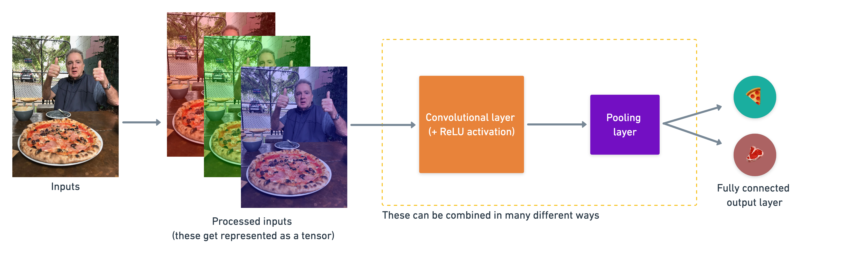 A simple example of how you might stack together the above layers into a convolutional neural network. Note the convolutional and pooling layers can often be arranged and rearranged into many different formations.
An end-to-end example
We've checked out our data and found there's 750 training images, as well as 250 test images per class and they're all of various different shapes.
It's time to jump straight in the deep end.
Reading the original dataset authors paper, we see they used a Random Forest machine learning model and averaged 50.76% accuracy at predicting what different foods different images had in them.
From now on, that 50.76% will be our baseline.
🔑 Note: A baseline is a score or evaluation metric you want to try and beat. Usually you'll start with a simple model, create a baseline and try to beat it by increasing the complexity of the model. A really fun way to learn machine learning is to find some kind of modelling paper with a published result and try to beat it.
The code in the following cell replicates and end-to-end way to model our pizza_steak dataset with a convolutional neural network (CNN) using the components listed above.
There will be a bunch of things you might not recognize but step through the code yourself and see if you can figure out what it's doing.
We'll go through each of the steps later on in the notebook.
For reference, the model we're using replicates TinyVGG, the computer vision architecture which fuels the CNN explainer webpage.
📖 Resource: The architecture we're using below is a scaled-down version of VGG-16, a convolutional neural network which came 2nd in the 2014 ImageNet classification competition.
import tensorflow as tf
from tensorflow.keras.preprocessing.image import ImageDataGenerator
# Set the seed
tf.random.set_seed(42)
# Preprocess data (get all of the pixel values between 1 and 0, also called scaling/normalization)
train_datagen = ImageDataGenerator(rescale=1./255)
valid_datagen = ImageDataGenerator(rescale=1./255)
# Setup the train and test directories
train_dir = "pizza_steak/train/"
test_dir = "pizza_steak/test/"
# Import data from directories and turn it into batches
train_data = train_datagen.flow_from_directory(train_dir,
batch_size=32, # number of images to process at a time
target_size=(224, 224), # convert all images to be 224 x 224
class_mode="binary", # type of problem we're working on
seed=42)
valid_data = valid_datagen.flow_from_directory(test_dir,
batch_size=32,
target_size=(224, 224),
class_mode="binary",
seed=42)
# Create a CNN model (same as Tiny VGG - https://poloclub.github.io/cnn-explainer/)
model_1 = tf.keras.models.Sequential([
tf.keras.layers.Conv2D(filters=10,
kernel_size=3, # can also be (3, 3)
activation="relu",
input_shape=(224, 224, 3)), # first layer specifies input shape (height, width, colour channels)
tf.keras.layers.Conv2D(10, 3, activation="relu"),
tf.keras.layers.MaxPool2D(pool_size=2, # pool_size can also be (2, 2)
padding="valid"), # padding can also be 'same'
tf.keras.layers.Conv2D(10, 3, activation="relu"),
tf.keras.layers.Conv2D(10, 3, activation="relu"), # activation='relu' == tf.keras.layers.Activations(tf.nn.relu)
tf.keras.layers.MaxPool2D(2),
tf.keras.layers.Flatten(),
tf.keras.layers.Dense(1, activation="sigmoid") # binary activation output
])
# Compile the model
model_1.compile(loss="binary_crossentropy",
optimizer=tf.keras.optimizers.Adam(),
metrics=["accuracy"])
# Fit the model
history_1 = model_1.fit(train_data,
epochs=5,
steps_per_epoch=len(train_data),
validation_data=valid_data,
validation_steps=len(valid_data))
Found 1500 images belonging to 2 classes. Found 500 images belonging to 2 classes. Epoch 1/5 47/47 [==============================] - 23s 209ms/step - loss: 0.5981 - accuracy: 0.6773 - val_loss: 0.4158 - val_accuracy: 0.8060 Epoch 2/5 47/47 [==============================] - 9s 194ms/step - loss: 0.4584 - accuracy: 0.7967 - val_loss: 0.3675 - val_accuracy: 0.8500 Epoch 3/5 47/47 [==============================] - 9s 192ms/step - loss: 0.4656 - accuracy: 0.7893 - val_loss: 0.4424 - val_accuracy: 0.7940 Epoch 4/5 47/47 [==============================] - 9s 192ms/step - loss: 0.4098 - accuracy: 0.8380 - val_loss: 0.3485 - val_accuracy: 0.8780 Epoch 5/5 47/47 [==============================] - 9s 191ms/step - loss: 0.3708 - accuracy: 0.8453 - val_loss: 0.3162 - val_accuracy: 0.8820
🤔 Note: If the cell above takes more than ~12 seconds per epoch to run, you might not be using a GPU accelerator. If you're using a Colab notebook, you can access a GPU accelerator by going to Runtime -> Change Runtime Type -> Hardware Accelerator and select "GPU". After doing so, you might have to rerun all of the above cells as changing the runtime type causes Colab to have to reset.
Nice! After 5 epochs, our model beat the baseline score of 50.76% accuracy (our model got ~85% accuaracy on the training set and ~85% accuracy on the test set).
However, our model only went through a binary classificaiton problem rather than all of the 101 classes in the Food101 dataset, so we can't directly compare these metrics. That being said, the results so far show that our model is learning something.
🛠 Practice: Step through each of the main blocks of code in the cell above, what do you think each is doing? It's okay if you're not sure, we'll go through this soon. In the meantime, spend 10-minutes playing around the incredible CNN explainer website. What do you notice about the layer names at the top of the webpage?
Since we've already fit a model, let's check out its architecture.
# Check out the layers in our model
model_1.summary()
Model: "sequential"
_________________________________________________________________
Layer (type) Output Shape Param #
=================================================================
conv2d (Conv2D) (None, 222, 222, 10) 280
conv2d_1 (Conv2D) (None, 220, 220, 10) 910
max_pooling2d (MaxPooling2D (None, 110, 110, 10) 0
)
conv2d_2 (Conv2D) (None, 108, 108, 10) 910
conv2d_3 (Conv2D) (None, 106, 106, 10) 910
max_pooling2d_1 (MaxPooling (None, 53, 53, 10) 0
2D)
flatten (Flatten) (None, 28090) 0
dense (Dense) (None, 1) 28091
=================================================================
Total params: 31,101
Trainable params: 31,101
Non-trainable params: 0
_________________________________________________________________
What do you notice about the names of model_1's layers and the layer names at the top of the CNN explainer website?
I'll let you in on a little secret: we've replicated the exact architecture they use for their model demo.
Look at you go! You're already starting to replicate models you find in the wild.
Now there are a few new things here we haven't discussed, namely:
- The
ImageDataGeneratorclass and therescaleparameter - The
flow_from_directory()method- The
batch_sizeparameter - The
target_sizeparameter
- The
Conv2Dlayers (and the parameters which come with them)MaxPool2Dlayers (and their parameters).- The
steps_per_epochandvalidation_stepsparameters in thefit()function
Before we dive into each of these, let's see what happens if we try to fit a model we've worked with previously to our data.
Using the same model as before
To examplify how neural networks can be adapted to many different problems, let's see how a binary classification model we've previously built might work with our data.
🔑 Note: If you haven't gone through the previous classification notebook, no troubles, we'll be bringing in the a simple 4 layer architecture used to separate dots replicated from the TensorFlow Playground environment.
We can use all of the same parameters in our previous model except for changing two things:
- The data - we're now working with images instead of dots.
- The input shape - we have to tell our neural network the shape of the images we're working with.
- A common practice is to reshape images all to one size. In our case, we'll resize the images to
(224, 224, 3), meaning a height and width of 224 pixels and a depth of 3 for the red, green, blue colour channels.
- A common practice is to reshape images all to one size. In our case, we'll resize the images to
# Set random seed
tf.random.set_seed(42)
# Create a model to replicate the TensorFlow Playground model
model_2 = tf.keras.Sequential([
tf.keras.layers.Flatten(input_shape=(224, 224, 3)), # dense layers expect a 1-dimensional vector as input
tf.keras.layers.Dense(4, activation='relu'),
tf.keras.layers.Dense(4, activation='relu'),
tf.keras.layers.Dense(1, activation='sigmoid')
])
# Compile the model
model_2.compile(loss='binary_crossentropy',
optimizer=tf.keras.optimizers.Adam(),
metrics=["accuracy"])
# Fit the model
history_2 = model_2.fit(train_data, # use same training data created above
epochs=5,
steps_per_epoch=len(train_data),
validation_data=valid_data, # use same validation data created above
validation_steps=len(valid_data))
Epoch 1/5 47/47 [==============================] - 11s 197ms/step - loss: 1.7892 - accuracy: 0.4920 - val_loss: 0.6932 - val_accuracy: 0.5000 Epoch 2/5 47/47 [==============================] - 9s 191ms/step - loss: 0.6932 - accuracy: 0.5000 - val_loss: 0.6932 - val_accuracy: 0.5000 Epoch 3/5 47/47 [==============================] - 9s 189ms/step - loss: 0.6932 - accuracy: 0.5000 - val_loss: 0.6932 - val_accuracy: 0.5000 Epoch 4/5 47/47 [==============================] - 9s 199ms/step - loss: 0.6932 - accuracy: 0.5000 - val_loss: 0.6931 - val_accuracy: 0.5000 Epoch 5/5 47/47 [==============================] - 9s 196ms/step - loss: 0.6932 - accuracy: 0.5000 - val_loss: 0.6931 - val_accuracy: 0.5000
Hmmm... our model ran but it doesn't seem like it learned anything. It only reaches 50% accuracy on the training and test sets which in a binary classification problem is as good as guessing.
Let's see the architecture.
# Check out our second model's architecture
model_2.summary()
Model: "sequential_1"
_________________________________________________________________
Layer (type) Output Shape Param #
=================================================================
flatten_1 (Flatten) (None, 150528) 0
dense_1 (Dense) (None, 4) 602116
dense_2 (Dense) (None, 4) 20
dense_3 (Dense) (None, 1) 5
=================================================================
Total params: 602,141
Trainable params: 602,141
Non-trainable params: 0
_________________________________________________________________
Wow. One of the most noticeable things here is the much larger number of parameters in model_2 versus model_1.
model_2 has 602,141 trainable parameters where as model_1 has only 31,101. And despite this difference, model_1 still far and large out performs model_2.
🔑 Note: You can think of trainable parameters as patterns a model can learn from data. Intuitiely, you might think more is better. And in some cases it is. But in this case, the difference here is in the two different styles of model we're using. Where a series of dense layers have a number of different learnable parameters connected to each other and hence a higher number of possible learnable patterns, a convolutional neural network seeks to sort out and learn the most important patterns in an image. So even though there are less learnable parameters in our convolutional neural network, these are often more helpful in decphering between different features in an image.
Since our previous model didn't work, do you have any ideas of how we might make it work?
How about we increase the number of layers?
And maybe even increase the number of neurons in each layer?
More specifically, we'll increase the number of neurons (also called hidden units) in each dense layer from 4 to 100 and add an extra layer.
🔑 Note: Adding extra layers or increasing the number of neurons in each layer is often referred to as increasing the complexity of your model.
# Set random seed
tf.random.set_seed(42)
# Create a model similar to model_1 but add an extra layer and increase the number of hidden units in each layer
model_3 = tf.keras.Sequential([
tf.keras.layers.Flatten(input_shape=(224, 224, 3)), # dense layers expect a 1-dimensional vector as input
tf.keras.layers.Dense(100, activation='relu'), # increase number of neurons from 4 to 100 (for each layer)
tf.keras.layers.Dense(100, activation='relu'),
tf.keras.layers.Dense(100, activation='relu'), # add an extra layer
tf.keras.layers.Dense(1, activation='sigmoid')
])
# Compile the model
model_3.compile(loss='binary_crossentropy',
optimizer=tf.keras.optimizers.Adam(),
metrics=["accuracy"])
# Fit the model
history_3 = model_3.fit(train_data,
epochs=5,
steps_per_epoch=len(train_data),
validation_data=valid_data,
validation_steps=len(valid_data))
Epoch 1/5 47/47 [==============================] - 11s 201ms/step - loss: 2.8247 - accuracy: 0.6413 - val_loss: 0.6214 - val_accuracy: 0.7720 Epoch 2/5 47/47 [==============================] - 9s 195ms/step - loss: 0.6881 - accuracy: 0.7300 - val_loss: 0.5762 - val_accuracy: 0.7140 Epoch 3/5 47/47 [==============================] - 9s 196ms/step - loss: 1.2195 - accuracy: 0.6860 - val_loss: 0.6234 - val_accuracy: 0.7320 Epoch 4/5 47/47 [==============================] - 9s 194ms/step - loss: 0.5172 - accuracy: 0.7893 - val_loss: 0.5061 - val_accuracy: 0.7600 Epoch 5/5 47/47 [==============================] - 9s 192ms/step - loss: 0.5041 - accuracy: 0.7833 - val_loss: 0.4380 - val_accuracy: 0.8000
Woah! Looks like our model is learning again. It got ~70% accuracy on the training set and ~70% accuracy on the validation set.
How does the architecute look?
# Check out model_3 architecture
model_3.summary()
Model: "sequential_2"
_________________________________________________________________
Layer (type) Output Shape Param #
=================================================================
flatten_2 (Flatten) (None, 150528) 0
dense_4 (Dense) (None, 100) 15052900
dense_5 (Dense) (None, 100) 10100
dense_6 (Dense) (None, 100) 10100
dense_7 (Dense) (None, 1) 101
=================================================================
Total params: 15,073,201
Trainable params: 15,073,201
Non-trainable params: 0
_________________________________________________________________
My gosh, the number of trainable parameters has increased even more than model_2. And even with close to 500x (~15,000,000 vs. ~31,000) more trainable parameters, model_3 still doesn't out perform model_1.
This goes to show the power of convolutional neural networks and their ability to learn patterns despite using less parameters.
Binary classification: Let's break it down
We just went through a whirlwind of steps:
- Become one with the data (visualize, visualize, visualize...)
- Preprocess the data (prepare it for a model)
- Create a model (start with a baseline)
- Fit the model
- Evaluate the model
- Adjust different parameters and improve model (try to beat your baseline)
- Repeat until satisfied
Let's step through each.
1. Import and become one with the data
Whatever kind of data you're dealing with, it's a good idea to visualize at least 10-100 samples to start to building your own mental model of the data.
In our case, we might notice that the steak images tend to have darker colours where as pizza images tend to have a distinct circular shape in the middle. These might be patterns that our neural network picks up on.
You an also notice if some of your data is messed up (for example, has the wrong label) and start to consider ways you might go about fixing it.
📖 Resource: To see how this data was processed into the file format we're using, see the preprocessing notebook.
If the visualization cell below doesn't work, make sure you've got the data by uncommenting the cell below.
# import zipfile
# # Download zip file of pizza_steak images
# !wget https://storage.googleapis.com/ztm_tf_course/food_vision/pizza_steak.zip
# # Unzip the downloaded file
# zip_ref = zipfile.ZipFile("pizza_steak.zip", "r")
# zip_ref.extractall()
# zip_ref.close()
# Visualize data (requires function 'view_random_image' above)
plt.figure()
plt.subplot(1, 2, 1)
steak_img = view_random_image("pizza_steak/train/", "steak")
plt.subplot(1, 2, 2)
pizza_img = view_random_image("pizza_steak/train/", "pizza")
Image shape: (512, 512, 3) Image shape: (512, 512, 3)

2. Preprocess the data (prepare it for a model)
One of the most important steps for a machine learning project is creating a training and test set.
In our case, our data is already split into training and test sets. Another option here might be to create a validation set as well, but we'll leave that for now.
For an image classification project, it's standard to have your data seperated into train and test directories with subfolders in each for each class.
To start we define the training and test directory paths.
# Define training and test directory paths
train_dir = "pizza_steak/train/"
test_dir = "pizza_steak/test/"
Our next step is to turn our data into batches.
A batch is a small subset of the dataset a model looks at during training. For example, rather than looking at 10,000 images at one time and trying to figure out the patterns, a model might only look at 32 images at a time.
It does this for a couple of reasons:
- 10,000 images (or more) might not fit into the memory of your processor (GPU).
- Trying to learn the patterns in 10,000 images in one hit could result in the model not being able to learn very well.
Why 32?
A batch size of 32 is good for your health.
No seriously, there are many different batch sizes you could use but 32 has proven to be very effective in many different use cases and is often the default for many data preprocessing functions.
To turn our data into batches, we'll first create an instance of ImageDataGenerator for each of our datasets.
# Create train and test data generators and rescale the data
from tensorflow.keras.preprocessing.image import ImageDataGenerator
train_datagen = ImageDataGenerator(rescale=1/255.)
test_datagen = ImageDataGenerator(rescale=1/255.)
The ImageDataGenerator class helps us prepare our images into batches as well as perform transformations on them as they get loaded into the model.
You might've noticed the rescale parameter. This is one example of the transformations we're doing.
Remember from before how we imported an image and it's pixel values were between 0 and 255?
The rescale parameter, along with 1/255. is like saying "divide all of the pixel values by 255". This results in all of the image being imported and their pixel values being normalized (converted to be between 0 and 1).
🔑 Note: For more transformation options such as data augmentation (we'll see this later), refer to the
ImageDataGeneratordocumentation.
Now we've got a couple of ImageDataGenerator instances, we can load our images from their respective directories using the flow_from_directory method.
# Turn it into batches
train_data = train_datagen.flow_from_directory(directory=train_dir,
target_size=(224, 224),
class_mode='binary',
batch_size=32)
test_data = test_datagen.flow_from_directory(directory=test_dir,
target_size=(224, 224),
class_mode='binary',
batch_size=32)
Found 1500 images belonging to 2 classes. Found 500 images belonging to 2 classes.
Wonderful! Looks like our training dataset has 1500 images belonging to 2 classes (pizza and steak) and our test dataset has 500 images also belonging to 2 classes.
Some things to here:
- Due to how our directories are structured, the classes get inferred by the subdirectory names in
train_dirandtest_dir. - The
target_sizeparameter defines the input size of our images in(height, width)format. - The
class_modevalue of'binary'defines our classification problem type. If we had more than two classes, we would use'categorical'. - The
batch_sizedefines how many images will be in each batch, we've used 32 which is the same as the default.
We can take a look at our batched images and labels by inspecting the train_data object.
# Get a sample of the training data batch
images, labels = train_data.next() # get the 'next' batch of images/labels
len(images), len(labels)
(32, 32)
Wonderful, it seems our images and labels are in batches of 32.
Let's see what the images look like.
# Get the first two images
images[:2], images[0].shape
(array([[[[0.47058827, 0.40784317, 0.34509805],
[0.4784314 , 0.427451 , 0.3647059 ],
[0.48627454, 0.43529415, 0.37254903],
...,
[0.8313726 , 0.70980394, 0.48627454],
[0.8431373 , 0.73333335, 0.5372549 ],
[0.87843144, 0.7725491 , 0.5882353 ]],
[[0.50980395, 0.427451 , 0.36078432],
[0.5058824 , 0.42352945, 0.35686275],
[0.5137255 , 0.4431373 , 0.3647059 ],
...,
[0.82745105, 0.7058824 , 0.48235297],
[0.82745105, 0.70980394, 0.5058824 ],
[0.8431373 , 0.73333335, 0.5372549 ]],
[[0.5254902 , 0.427451 , 0.34901962],
[0.5372549 , 0.43921572, 0.36078432],
[0.5372549 , 0.45098042, 0.36078432],
...,
[0.82745105, 0.7019608 , 0.4784314 ],
[0.82745105, 0.7058824 , 0.49411768],
[0.8352942 , 0.7176471 , 0.5137255 ]],
...,
[[0.77647066, 0.5647059 , 0.2901961 ],
[0.7803922 , 0.53333336, 0.22352943],
[0.79215693, 0.5176471 , 0.18039216],
...,
[0.30588236, 0.2784314 , 0.24705884],
[0.24705884, 0.23137257, 0.19607845],
[0.2784314 , 0.27450982, 0.25490198]],
[[0.7843138 , 0.57254905, 0.29803923],
[0.79215693, 0.54509807, 0.24313727],
[0.8000001 , 0.5254902 , 0.18823531],
...,
[0.2627451 , 0.23529413, 0.20392159],
[0.24313727, 0.227451 , 0.19215688],
[0.26666668, 0.2627451 , 0.24313727]],
[[0.7960785 , 0.59607846, 0.3372549 ],
[0.7960785 , 0.5647059 , 0.26666668],
[0.81568635, 0.54901963, 0.22352943],
...,
[0.23529413, 0.19607845, 0.16078432],
[0.3019608 , 0.26666668, 0.24705884],
[0.26666668, 0.2509804 , 0.24705884]]],
[[[0.38823533, 0.4666667 , 0.36078432],
[0.3921569 , 0.46274513, 0.36078432],
[0.38431376, 0.454902 , 0.36078432],
...,
[0.5294118 , 0.627451 , 0.54509807],
[0.5294118 , 0.627451 , 0.54509807],
[0.5411765 , 0.6392157 , 0.5568628 ]],
[[0.38431376, 0.454902 , 0.3529412 ],
[0.3921569 , 0.46274513, 0.36078432],
[0.39607847, 0.4666667 , 0.37254903],
...,
[0.54509807, 0.6431373 , 0.5686275 ],
[0.5529412 , 0.6509804 , 0.5764706 ],
[0.5647059 , 0.6627451 , 0.5882353 ]],
[[0.3921569 , 0.46274513, 0.36078432],
[0.38431376, 0.454902 , 0.3529412 ],
[0.4039216 , 0.47450984, 0.3803922 ],
...,
[0.5764706 , 0.67058825, 0.6156863 ],
[0.5647059 , 0.6666667 , 0.6156863 ],
[0.5647059 , 0.6666667 , 0.6156863 ]],
...,
[[0.47058827, 0.5647059 , 0.4784314 ],
[0.4784314 , 0.5764706 , 0.4901961 ],
[0.48235297, 0.5803922 , 0.49803925],
...,
[0.39607847, 0.42352945, 0.3019608 ],
[0.37647063, 0.40000004, 0.2901961 ],
[0.3803922 , 0.4039216 , 0.3019608 ]],
[[0.45098042, 0.5529412 , 0.454902 ],
[0.46274513, 0.5647059 , 0.4666667 ],
[0.47058827, 0.57254905, 0.47450984],
...,
[0.40784317, 0.43529415, 0.3137255 ],
[0.39607847, 0.41960788, 0.31764707],
[0.38823533, 0.40784317, 0.31764707]],
[[0.47450984, 0.5764706 , 0.47058827],
[0.47058827, 0.57254905, 0.4666667 ],
[0.46274513, 0.5647059 , 0.4666667 ],
...,
[0.4039216 , 0.427451 , 0.31764707],
[0.3921569 , 0.4156863 , 0.3137255 ],
[0.4039216 , 0.42352945, 0.3372549 ]]]], dtype=float32),
(224, 224, 3))
Due to our rescale parameter, the images are now in (224, 224, 3) shape tensors with values between 0 and 1.
How about the labels?
# View the first batch of labels
labels
array([1., 1., 0., 1., 0., 0., 0., 1., 0., 1., 0., 0., 1., 0., 0., 0., 1.,
1., 0., 1., 0., 1., 1., 1., 0., 0., 0., 0., 0., 1., 0., 1.],
dtype=float32)
Due to the class_mode parameter being 'binary' our labels are either 0 (pizza) or 1 (steak).
Now that our data is ready, our model is going to try and figure out the patterns between the image tensors and the labels.
3. Create a model (start with a baseline)
You might be wondering what your default model architecture should be.
And the truth is, there's many possible answers to this question.
A simple heuristic for computer vision models is to use the model architecture which is performing best on ImageNet (a large collection of diverse images to benchmark different computer vision models).
However, to begin with, it's good to build a smaller model to acquire a baseline result which you try to improve upon.
🔑 Note: In deep learning a smaller model often refers to a model with less layers than the state of the art (SOTA). For example, a smaller model might have 3-4 layers where as a state of the art model, such as, ResNet50 might have 50+ layers.
In our case, let's take a smaller version of the model that can be found on the CNN explainer website (model_1 from above) and build a 3 layer convolutional neural network.
# Make the creating of our model a little easier
from tensorflow.keras.optimizers import Adam
from tensorflow.keras.layers import Dense, Flatten, Conv2D, MaxPool2D, Activation
from tensorflow.keras import Sequential
# Create the model (this can be our baseline, a 3 layer Convolutional Neural Network)
model_4 = Sequential([
Conv2D(filters=10,
kernel_size=3,
strides=1,
padding='valid',
activation='relu',
input_shape=(224, 224, 3)), # input layer (specify input shape)
Conv2D(10, 3, activation='relu'),
Conv2D(10, 3, activation='relu'),
Flatten(),
Dense(1, activation='sigmoid') # output layer (specify output shape)
])
Great! We've got a simple convolutional neural network architecture ready to go.
And it follows the typical CNN structure of:
Input -> Conv + ReLU layers (non-linearities) -> Pooling layer -> Fully connected (dense layer) as Output
Let's discuss some of the components of the Conv2D layer:
- The "
2D" means our inputs are two dimensional (height and width), even though they have 3 colour channels, the convolutions are run on each channel invididually. filters- these are the number of "feature extractors" that will be moving over our images.kernel_size- the size of our filters, for example, akernel_sizeof(3, 3)(or just 3) will mean each filter will have the size 3x3, meaning it will look at a space of 3x3 pixels each time. The smaller the kernel, the more fine-grained features it will extract.stride- the number of pixels afilterwill move across as it covers the image. Astrideof 1 means the filter moves across each pixel 1 by 1. Astrideof 2 means it moves 2 pixels at a time.padding- this can be either'same'or'valid','same'adds zeros the to outside of the image so the resulting output of the convolutional layer is the same as the input, where as'valid'(default) cuts off excess pixels where thefilterdoesn't fit (e.g. 224 pixels wide divided by a kernel size of 3 (224/3 = 74.6) means a single pixel will get cut off the end.
What's a "feature"?
A feature can be considered any significant part of an image. For example, in our case, a feature might be the circular shape of pizza. Or the rough edges on the outside of a steak.
It's important to note that these features are not defined by us, instead, the model learns them as it applies different filters across the image.
📖 Resources: For a great demonstration of these in action, be sure to spend some time going through the following:
- CNN Explainer Webpage - a great visual overview of many of the concepts we're replicating here with code.
- A guide to convolutional arithmetic for deep learning - a phenomenal introduction to the math going on behind the scenes of a convolutional neural network.
- For a great explanation of padding, see this Stack Overflow answer.
Now our model is ready, let's compile it.
# Compile the model
model_4.compile(loss='binary_crossentropy',
optimizer=Adam(),
metrics=['accuracy'])
Since we're working on a binary classification problem (pizza vs. steak), the loss function we're using is 'binary_crossentropy', if it was mult-iclass, we might use something like 'categorical_crossentropy'.
Adam with all the default settings is our optimizer and our evaluation metric is accuracy.
4. Fit a model
Our model is compiled, time to fit it.
You'll notice two new parameters here:
steps_per_epoch- this is the number of batches a model will go through per epoch, in our case, we want our model to go through all batches so it's equal to the length oftrain_data(1500 images in batches of 32 = 1500/32 = ~47 steps)validation_steps- same as above, except for thevalidation_dataparameter (500 test images in batches of 32 = 500/32 = ~16 steps)
# Check lengths of training and test data generators
len(train_data), len(test_data)
(47, 16)
# Fit the model
history_4 = model_4.fit(train_data,
epochs=5,
steps_per_epoch=len(train_data),
validation_data=test_data,
validation_steps=len(test_data))
Epoch 1/5 47/47 [==============================] - 11s 198ms/step - loss: 0.6262 - accuracy: 0.6733 - val_loss: 0.4172 - val_accuracy: 0.8140 Epoch 2/5 47/47 [==============================] - 9s 192ms/step - loss: 0.4260 - accuracy: 0.8253 - val_loss: 0.3766 - val_accuracy: 0.8420 Epoch 3/5 47/47 [==============================] - 9s 191ms/step - loss: 0.2717 - accuracy: 0.9100 - val_loss: 0.3451 - val_accuracy: 0.8580 Epoch 4/5 47/47 [==============================] - 9s 191ms/step - loss: 0.1141 - accuracy: 0.9720 - val_loss: 0.3705 - val_accuracy: 0.8440 Epoch 5/5 47/47 [==============================] - 9s 191ms/step - loss: 0.0478 - accuracy: 0.9900 - val_loss: 0.5217 - val_accuracy: 0.8220
5. Evaluate the model
Oh yeah! Looks like our model is learning something.
Let's check out its training curves.
# Plot the training curves
import pandas as pd
pd.DataFrame(history_4.history).plot(figsize=(10, 7));

Hmm, judging by our loss curves, it looks like our model is overfitting the training dataset.
🔑 Note: When a model's validation loss starts to increase, it's likely that it's overfitting the training dataset. This means, it's learning the patterns in the training dataset too well and thus its ability to generalize to unseen data will be diminished.
To further inspect our model's training performance, let's separate the accuracy and loss curves.
# Plot the validation and training data separately
def plot_loss_curves(history):
"""
Returns separate loss curves for training and validation metrics.
"""
loss = history.history['loss']
val_loss = history.history['val_loss']
accuracy = history.history['accuracy']
val_accuracy = history.history['val_accuracy']
epochs = range(len(history.history['loss']))
# Plot loss
plt.plot(epochs, loss, label='training_loss')
plt.plot(epochs, val_loss, label='val_loss')
plt.title('Loss')
plt.xlabel('Epochs')
plt.legend()
# Plot accuracy
plt.figure()
plt.plot(epochs, accuracy, label='training_accuracy')
plt.plot(epochs, val_accuracy, label='val_accuracy')
plt.title('Accuracy')
plt.xlabel('Epochs')
plt.legend();
# Check out the loss curves of model_4
plot_loss_curves(history_4)


The ideal position for these two curves is to follow each other. If anything, the validation curve should be slightly under the training curve. If there's a large gap between the training curve and validation curve, it means your model is probably overfitting.
# Check out our model's architecture
model_4.summary()
Model: "sequential_3"
_________________________________________________________________
Layer (type) Output Shape Param #
=================================================================
conv2d_4 (Conv2D) (None, 222, 222, 10) 280
conv2d_5 (Conv2D) (None, 220, 220, 10) 910
conv2d_6 (Conv2D) (None, 218, 218, 10) 910
flatten_3 (Flatten) (None, 475240) 0
dense_8 (Dense) (None, 1) 475241
=================================================================
Total params: 477,341
Trainable params: 477,341
Non-trainable params: 0
_________________________________________________________________
6. Adjust the model parameters
Fitting a machine learning model comes in 3 steps: 0. Create a basline.
- Beat the baseline by overfitting a larger model.
- Reduce overfitting.
So far we've gone through steps 0 and 1.
And there are even a few more things we could try to further overfit our model:
- Increase the number of convolutional layers.
- Increase the number of convolutional filters.
- Add another dense layer to the output of our flattened layer.
But what we'll do instead is focus on getting our model's training curves to better align with eachother, in other words, we'll take on step 2.
Why is reducing overfitting important?
When a model performs too well on training data and poorly on unseen data, it's not much use to us if we wanted to use it in the real world.
Say we were building a pizza vs. steak food classifier app, and our model performs very well on our training data but when users tried it out, they didn't get very good results on their own food images, is that a good experience?
Not really...
So for the next few models we build, we're going to adjust a number of parameters and inspect the training curves along the way.
Namely, we'll build 2 more models:
- A ConvNet with max pooling
- A ConvNet with max pooling and data augmentation
For the first model, we'll follow the modified basic CNN structure:
Input -> Conv layers + ReLU layers (non-linearities) + Max Pooling layers -> Fully connected (dense layer) as Output
Let's built it. It'll have the same structure as model_4 but with a MaxPool2D() layer after each convolutional layer.
# Create the model (this can be our baseline, a 3 layer Convolutional Neural Network)
model_5 = Sequential([
Conv2D(10, 3, activation='relu', input_shape=(224, 224, 3)),
MaxPool2D(pool_size=2), # reduce number of features by half
Conv2D(10, 3, activation='relu'),
MaxPool2D(),
Conv2D(10, 3, activation='relu'),
MaxPool2D(),
Flatten(),
Dense(1, activation='sigmoid')
])
Woah, we've got another layer type we haven't seen before.
If convolutional layers learn the features of an image you can think of a Max Pooling layer as figuring out the most important of those features. We'll see this an example of this in a moment.
# Compile model (same as model_4)
model_5.compile(loss='binary_crossentropy',
optimizer=Adam(),
metrics=['accuracy'])
# Fit the model
history_5 = model_5.fit(train_data,
epochs=5,
steps_per_epoch=len(train_data),
validation_data=test_data,
validation_steps=len(test_data))
Epoch 1/5 47/47 [==============================] - 11s 196ms/step - loss: 0.6482 - accuracy: 0.6240 - val_loss: 0.5451 - val_accuracy: 0.7100 Epoch 2/5 47/47 [==============================] - 9s 190ms/step - loss: 0.4537 - accuracy: 0.8013 - val_loss: 0.3536 - val_accuracy: 0.8380 Epoch 3/5 47/47 [==============================] - 9s 192ms/step - loss: 0.4161 - accuracy: 0.8233 - val_loss: 0.3578 - val_accuracy: 0.8460 Epoch 4/5 47/47 [==============================] - 9s 192ms/step - loss: 0.3903 - accuracy: 0.8353 - val_loss: 0.3509 - val_accuracy: 0.8480 Epoch 5/5 47/47 [==============================] - 9s 192ms/step - loss: 0.3567 - accuracy: 0.8513 - val_loss: 0.3200 - val_accuracy: 0.8700
Okay, it looks like our model with max pooling (model_5) is performing worse on the training set but better on the validation set.
Before we checkout its training curves, let's check out its architecture.
# Check out the model architecture
model_5.summary()
Model: "sequential_4"
_________________________________________________________________
Layer (type) Output Shape Param #
=================================================================
conv2d_7 (Conv2D) (None, 222, 222, 10) 280
max_pooling2d_2 (MaxPooling (None, 111, 111, 10) 0
2D)
conv2d_8 (Conv2D) (None, 109, 109, 10) 910
max_pooling2d_3 (MaxPooling (None, 54, 54, 10) 0
2D)
conv2d_9 (Conv2D) (None, 52, 52, 10) 910
max_pooling2d_4 (MaxPooling (None, 26, 26, 10) 0
2D)
flatten_4 (Flatten) (None, 6760) 0
dense_9 (Dense) (None, 1) 6761
=================================================================
Total params: 8,861
Trainable params: 8,861
Non-trainable params: 0
_________________________________________________________________
Do you notice what's going on here with the output shape in each MaxPooling2D layer?
It gets halved each time. This is effectively the MaxPooling2D layer taking the outputs of each Conv2D layer and saying "I only want the most important features, get rid of the rest".
The bigger the pool_size parameter, the more the max pooling layer will squeeze the features out of the image. However, too big and the model might not be able to learn anything.
The results of this pooling are seen in a major reduction of total trainable parameters (8,861 in model_5 and 477,431 in model_4).
Time to check out the loss curves.
# Plot loss curves of model_5 results
plot_loss_curves(history_5)


Nice! We can see the training curves get a lot closer to eachother. However, our the validation loss looks to start increasing towards the end and in turn potentially leading to overfitting.
Time to dig into our bag of tricks and try another method of overfitting prevention, data augmentation.
First, we'll see how it's done with code then we'll discuss what it's doing.
To implement data augmentation, we'll have to reinstantiate our ImageDataGenerator instances.
# Create ImageDataGenerator training instance with data augmentation
train_datagen_augmented = ImageDataGenerator(rescale=1/255.,
rotation_range=20, # rotate the image slightly between 0 and 20 degrees (note: this is an int not a float)
shear_range=0.2, # shear the image
zoom_range=0.2, # zoom into the image
width_shift_range=0.2, # shift the image width ways
height_shift_range=0.2, # shift the image height ways
horizontal_flip=True) # flip the image on the horizontal axis
# Create ImageDataGenerator training instance without data augmentation
train_datagen = ImageDataGenerator(rescale=1/255.)
# Create ImageDataGenerator test instance without data augmentation
test_datagen = ImageDataGenerator(rescale=1/255.)
🤔 Question: What's data augmentation?
Data augmentation is the process of altering our training data, leading to it having more diversity and in turn allowing our models to learn more generalizable patterns. Altering might mean adjusting the rotation of an image, flipping it, cropping it or something similar.
Doing this simulates the kind of data a model might be used on in the real world.
If we're building a pizza vs. steak application, not all of the images our users take might be in similar setups to our training data. Using data augmentation gives us another way to prevent overfitting and in turn make our model more generalizable.
🔑 Note: Data augmentation is usally only performed on the training data. Using the
ImageDataGeneratorbuilt-in data augmentation parameters our images are left as they are in the directories but are randomly manipulated when loaded into the model.
# Import data and augment it from training directory
print("Augmented training images:")
train_data_augmented = train_datagen_augmented.flow_from_directory(train_dir,
target_size=(224, 224),
batch_size=32,
class_mode='binary',
shuffle=False) # Don't shuffle for demonstration purposes, usually a good thing to shuffle
# Create non-augmented data batches
print("Non-augmented training images:")
train_data = train_datagen.flow_from_directory(train_dir,
target_size=(224, 224),
batch_size=32,
class_mode='binary',
shuffle=False) # Don't shuffle for demonstration purposes
print("Unchanged test images:")
test_data = test_datagen.flow_from_directory(test_dir,
target_size=(224, 224),
batch_size=32,
class_mode='binary')
Augmented training images: Found 1500 images belonging to 2 classes. Non-augmented training images: Found 1500 images belonging to 2 classes. Unchanged test images: Found 500 images belonging to 2 classes.
Better than talk about data augmentation, how about we see it?
(remember our motto? visualize, visualize, visualize...)
# Get data batch samples
images, labels = train_data.next()
augmented_images, augmented_labels = train_data_augmented.next() # Note: labels aren't augmented, they stay the same
# Show original image and augmented image
random_number = random.randint(0, 31) # we're making batches of size 32, so we'll get a random instance
plt.imshow(images[random_number])
plt.title(f"Original image")
plt.axis(False)
plt.figure()
plt.imshow(augmented_images[random_number])
plt.title(f"Augmented image")
plt.axis(False);


After going through a sample of original and augmented images, you can start to see some of the example transformations on the training images.
Notice how some of the augmented images look like slightly warped versions of the original image. This means our model will be forced to try and learn patterns in less-than-perfect images, which is often the case when using real-world images.
🤔 Question: Should I use data augmentation? And how much should I augment?
Data augmentation is a way to try and prevent a model overfitting. If your model is overfiting (e.g. the validation loss keeps increasing), you may want to try using data augmentation.
As for how much to data augment, there's no set practice for this. Best to check out the options in the ImageDataGenerator class and think about how a model in your use case might benefit from some data augmentation.
Now we've got augmented data, let's try and refit a model on it and see how it affects training.
We'll use the same model as model_5.
# Create the model (same as model_5)
model_6 = Sequential([
Conv2D(10, 3, activation='relu', input_shape=(224, 224, 3)),
MaxPool2D(pool_size=2), # reduce number of features by half
Conv2D(10, 3, activation='relu'),
MaxPool2D(),
Conv2D(10, 3, activation='relu'),
MaxPool2D(),
Flatten(),
Dense(1, activation='sigmoid')
])
# Compile the model
model_6.compile(loss='binary_crossentropy',
optimizer=Adam(),
metrics=['accuracy'])
# Fit the model
history_6 = model_6.fit(train_data_augmented, # changed to augmented training data
epochs=5,
steps_per_epoch=len(train_data_augmented),
validation_data=test_data,
validation_steps=len(test_data))
Epoch 1/5 47/47 [==============================] - 24s 472ms/step - loss: 0.8005 - accuracy: 0.4447 - val_loss: 0.7007 - val_accuracy: 0.5000 Epoch 2/5 47/47 [==============================] - 22s 475ms/step - loss: 0.6981 - accuracy: 0.4267 - val_loss: 0.6918 - val_accuracy: 0.5140 Epoch 3/5 47/47 [==============================] - 22s 474ms/step - loss: 0.6938 - accuracy: 0.5033 - val_loss: 0.6896 - val_accuracy: 0.5100 Epoch 4/5 47/47 [==============================] - 22s 477ms/step - loss: 0.6886 - accuracy: 0.5120 - val_loss: 0.6732 - val_accuracy: 0.5240 Epoch 5/5 47/47 [==============================] - 22s 477ms/step - loss: 0.7195 - accuracy: 0.5187 - val_loss: 0.6886 - val_accuracy: 0.5360
🤔 Question: Why didn't our model get very good results on the training set to begin with?
It's because when we created train_data_augmented we turned off data shuffling using shuffle=False which means our model only sees a batch of a single kind of images at a time.
For example, the pizza class gets loaded in first because it's the first class. Thus it's performance is measured on only a single class rather than both classes. The validation data performance improves steadily because it contains shuffled data.
Since we only set shuffle=False for demonstration purposes (so we could plot the same augmented and non-augmented image), we can fix this by setting shuffle=True on future data generators.
You may have also noticed each epoch taking longer when training with augmented data compared to when training with non-augmented data (~25s per epoch vs. ~10s per epoch).
This is because the ImageDataGenerator instance augments the data as it's loaded into the model. The benefit of this is that it leaves the original images unchanged. The downside is that it takes longer to load them in.
🔑 Note: One possible method to speed up dataset manipulation would be to look into TensorFlow's parrallel reads and buffered prefecting options.
# Check model's performance history training on augmented data
plot_loss_curves(history_6)


It seems our validation loss curve is heading in the right direction but it's a bit jumpy (the most ideal loss curve isn't too spiky but a smooth descent, however, a perfectly smooth loss curve is the equivalent of a fairytale).
Let's see what happens when we shuffle the augmented training data.
# Import data and augment it from directories
train_data_augmented_shuffled = train_datagen_augmented.flow_from_directory(train_dir,
target_size=(224, 224),
batch_size=32,
class_mode='binary',
shuffle=True) # Shuffle data (default)
Found 1500 images belonging to 2 classes.
# Create the model (same as model_5 and model_6)
model_7 = Sequential([
Conv2D(10, 3, activation='relu', input_shape=(224, 224, 3)),
MaxPool2D(),
Conv2D(10, 3, activation='relu'),
MaxPool2D(),
Conv2D(10, 3, activation='relu'),
MaxPool2D(),
Flatten(),
Dense(1, activation='sigmoid')
])
# Compile the model
model_7.compile(loss='binary_crossentropy',
optimizer=Adam(),
metrics=['accuracy'])
# Fit the model
history_7 = model_7.fit(train_data_augmented_shuffled, # now the augmented data is shuffled
epochs=5,
steps_per_epoch=len(train_data_augmented_shuffled),
validation_data=test_data,
validation_steps=len(test_data))
Epoch 1/5 47/47 [==============================] - 24s 474ms/step - loss: 0.6685 - accuracy: 0.5613 - val_loss: 0.5886 - val_accuracy: 0.6960 Epoch 2/5 47/47 [==============================] - 22s 478ms/step - loss: 0.5598 - accuracy: 0.7073 - val_loss: 0.4351 - val_accuracy: 0.7880 Epoch 3/5 47/47 [==============================] - 22s 477ms/step - loss: 0.4849 - accuracy: 0.7647 - val_loss: 0.4040 - val_accuracy: 0.8280 Epoch 4/5 47/47 [==============================] - 23s 487ms/step - loss: 0.4862 - accuracy: 0.7733 - val_loss: 0.4282 - val_accuracy: 0.8100 Epoch 5/5 47/47 [==============================] - 23s 486ms/step - loss: 0.4627 - accuracy: 0.7873 - val_loss: 0.3589 - val_accuracy: 0.8540
# Check model's performance history training on augmented data
plot_loss_curves(history_7)


Notice with model_7 how the performance on the training dataset improves almost immediately compared to model_6. This is because we shuffled the training data as we passed it to the model using the parameter shuffle=True in the flow_from_directory method.
This means the model was able to see examples of both pizza and steak images in each batch and in turn be evaluated on what it learned from both images rather than just one kind.
Also, our loss curves look a little bit smoother with shuffled data (comparing history_6 to history_7).
7. Repeat until satisified
We've trained a few model's on our dataset already and so far they're performing pretty good.
Since we've already beaten our baseline, there are a few things we could try to continue to improve our model:
- Increase the number of model layers (e.g. add more convolutional layers).
- Increase the number of filters in each convolutional layer (e.g. from 10 to 32, 64, or 128, these numbers aren't set in stone either, they are usually found through trial and error).
- Train for longer (more epochs).
- Finding an ideal learning rate.
- Get more data (give the model more opportunities to learn).
- Use transfer learning to leverage what another image model has learned and adjust it for our own use case.
Adjusting each of these settings (except for the last two) during model development is usually referred to as hyperparameter tuning.
You can think of hyperparameter tuning as simialr to adjusting the settings on your oven to cook your favourite dish. Although your oven does most of the cooking for you, you can help it by tweaking the dials.
Let's go back to right where we started and try our original model (model_1 or the TinyVGG architecture from CNN explainer).
# Create a CNN model (same as Tiny VGG but for binary classification - https://poloclub.github.io/cnn-explainer/ )
model_8 = Sequential([
Conv2D(10, 3, activation='relu', input_shape=(224, 224, 3)), # same input shape as our images
Conv2D(10, 3, activation='relu'),
MaxPool2D(),
Conv2D(10, 3, activation='relu'),
Conv2D(10, 3, activation='relu'),
MaxPool2D(),
Flatten(),
Dense(1, activation='sigmoid')
])
# Compile the model
model_8.compile(loss="binary_crossentropy",
optimizer=tf.keras.optimizers.Adam(),
metrics=["accuracy"])
# Fit the model
history_8 = model_8.fit(train_data_augmented_shuffled,
epochs=5,
steps_per_epoch=len(train_data_augmented_shuffled),
validation_data=test_data,
validation_steps=len(test_data))
Epoch 1/5 47/47 [==============================] - 25s 492ms/step - loss: 0.6345 - accuracy: 0.6267 - val_loss: 0.4843 - val_accuracy: 0.7500 Epoch 2/5 47/47 [==============================] - 23s 495ms/step - loss: 0.5293 - accuracy: 0.7327 - val_loss: 0.3829 - val_accuracy: 0.8400 Epoch 3/5 47/47 [==============================] - 23s 490ms/step - loss: 0.5296 - accuracy: 0.7360 - val_loss: 0.5177 - val_accuracy: 0.7160 Epoch 4/5 47/47 [==============================] - 22s 475ms/step - loss: 0.4971 - accuracy: 0.7560 - val_loss: 0.3477 - val_accuracy: 0.8600 Epoch 5/5 47/47 [==============================] - 22s 476ms/step - loss: 0.4670 - accuracy: 0.7927 - val_loss: 0.3511 - val_accuracy: 0.8540
🔑 Note: You might've noticed we used some slightly different code to build
model_8as compared tomodel_1. This is because of the imports we did before, such asfrom tensorflow.keras.layers import Conv2Dreduce the amount of code we had to write. Although the code is different, the architectures are the same.
# Check model_1 architecture (same as model_8)
model_1.summary()
Model: "sequential"
_________________________________________________________________
Layer (type) Output Shape Param #
=================================================================
conv2d (Conv2D) (None, 222, 222, 10) 280
conv2d_1 (Conv2D) (None, 220, 220, 10) 910
max_pooling2d (MaxPooling2D (None, 110, 110, 10) 0
)
conv2d_2 (Conv2D) (None, 108, 108, 10) 910
conv2d_3 (Conv2D) (None, 106, 106, 10) 910
max_pooling2d_1 (MaxPooling (None, 53, 53, 10) 0
2D)
flatten (Flatten) (None, 28090) 0
dense (Dense) (None, 1) 28091
=================================================================
Total params: 31,101
Trainable params: 31,101
Non-trainable params: 0
_________________________________________________________________
# Check model_8 architecture (same as model_1)
model_8.summary()
Model: "sequential_7"
_________________________________________________________________
Layer (type) Output Shape Param #
=================================================================
conv2d_16 (Conv2D) (None, 222, 222, 10) 280
conv2d_17 (Conv2D) (None, 220, 220, 10) 910
max_pooling2d_11 (MaxPoolin (None, 110, 110, 10) 0
g2D)
conv2d_18 (Conv2D) (None, 108, 108, 10) 910
conv2d_19 (Conv2D) (None, 106, 106, 10) 910
max_pooling2d_12 (MaxPoolin (None, 53, 53, 10) 0
g2D)
flatten_7 (Flatten) (None, 28090) 0
dense_12 (Dense) (None, 1) 28091
=================================================================
Total params: 31,101
Trainable params: 31,101
Non-trainable params: 0
_________________________________________________________________
Now let's check out our TinyVGG model's performance.
# Check out the TinyVGG model performance
plot_loss_curves(history_8)


# How does this training curve look compared to the one above?
plot_loss_curves(history_1)


Hmm, our training curves are looking good, but our model's performance on the training and test sets didn't improve much compared to the previous model.
Taking another loook at the training curves, it looks like our model's performance might improve if we trained it a little longer (more epochs).
Perhaps that's something you like to try?
Making a prediction with our trained model
What good is a trained model if you can't make predictions with it?
To really test it out, we'll upload a couple of our own images and see how the model goes.
First, let's remind ourselves of the classnames and view the image we're going to test on.
# Classes we're working with
print(class_names)
['pizza' 'steak']
The first test image we're going to use is a delicious steak I cooked the other day.
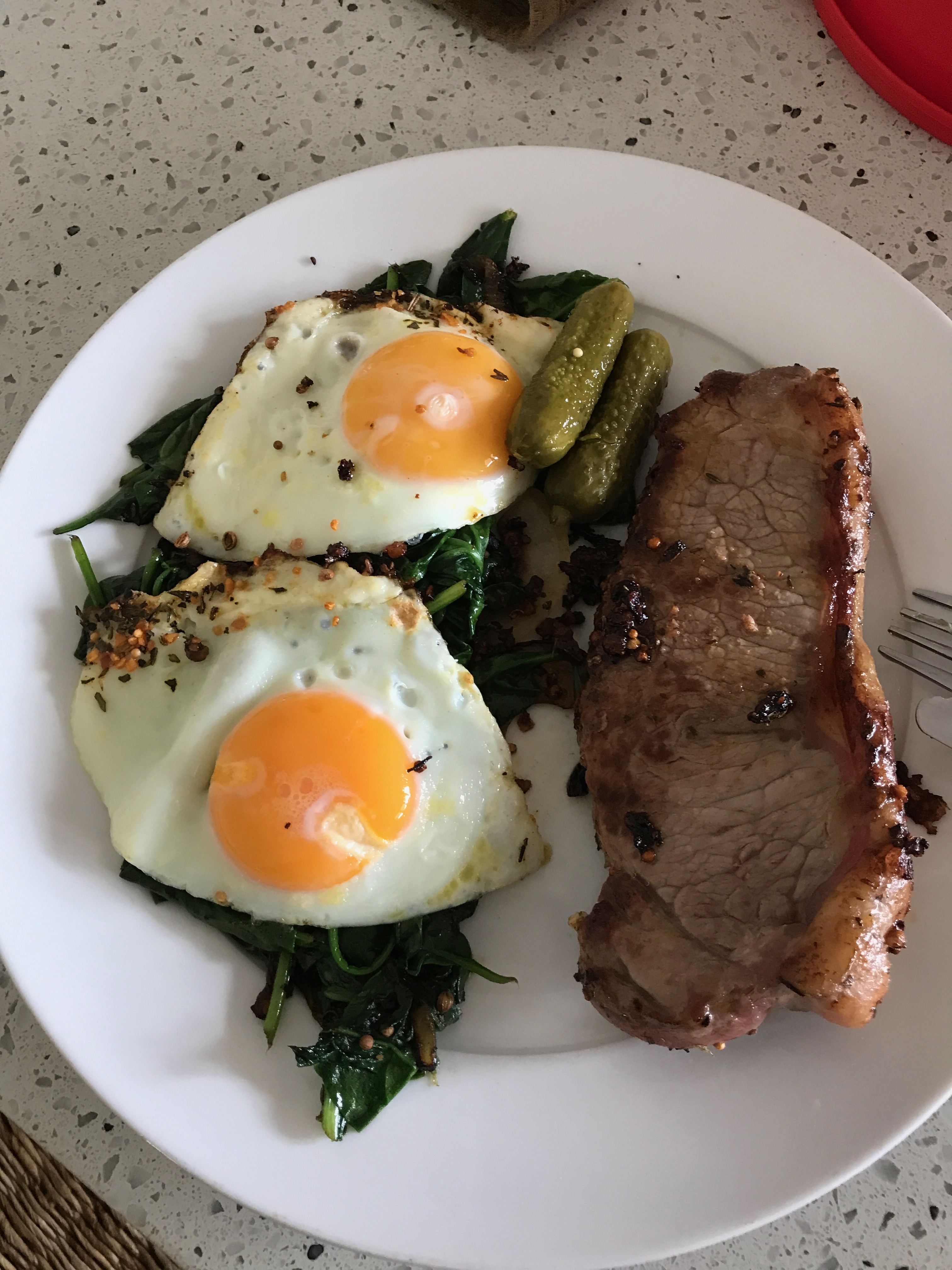
# View our example image
!wget https://raw.githubusercontent.com/mrdbourke/tensorflow-deep-learning/main/images/03-steak.jpeg
steak = mpimg.imread("03-steak.jpeg")
plt.imshow(steak)
plt.axis(False);
--2023-05-11 04:00:27-- https://raw.githubusercontent.com/mrdbourke/tensorflow-deep-learning/main/images/03-steak.jpeg Resolving raw.githubusercontent.com (raw.githubusercontent.com)... 185.199.108.133, 185.199.109.133, 185.199.110.133, ... Connecting to raw.githubusercontent.com (raw.githubusercontent.com)|185.199.108.133|:443... connected. HTTP request sent, awaiting response... 200 OK Length: 1978213 (1.9M) [image/jpeg] Saving to: ‘03-steak.jpeg’ 03-steak.jpeg 100%[===================>] 1.89M --.-KB/s in 0.02s 2023-05-11 04:00:27 (90.1 MB/s) - ‘03-steak.jpeg’ saved [1978213/1978213]

# Check the shape of our image
steak.shape
(4032, 3024, 3)
Since our model takes in images of shapes (224, 224, 3), we've got to reshape our custom image to use it with our model.
To do so, we can import and decode our image using tf.io.read_file (for readining files) and tf.image (for resizing our image and turning it into a tensor).
🔑 Note: For your model to make predictions on unseen data, for example, your own custom images, the custom image has to be in the same shape as your model has been trained on. In more general terms, to make predictions on custom data it has to be in the same form that your model has been trained on.
# Create a function to import an image and resize it to be able to be used with our model
def load_and_prep_image(filename, img_shape=224):
"""
Reads an image from filename, turns it into a tensor
and reshapes it to (img_shape, img_shape, colour_channel).
"""
# Read in target file (an image)
img = tf.io.read_file(filename)
# Decode the read file into a tensor & ensure 3 colour channels
# (our model is trained on images with 3 colour channels and sometimes images have 4 colour channels)
img = tf.image.decode_image(img, channels=3)
# Resize the image (to the same size our model was trained on)
img = tf.image.resize(img, size = [img_shape, img_shape])
# Rescale the image (get all values between 0 and 1)
img = img/255.
return img
Now we've got a function to load our custom image, let's load it in.
# Load in and preprocess our custom image
steak = load_and_prep_image("03-steak.jpeg")
steak
<tf.Tensor: shape=(224, 224, 3), dtype=float32, numpy=
array([[[0.6377451 , 0.6220588 , 0.57892156],
[0.6504902 , 0.63186276, 0.5897059 ],
[0.63186276, 0.60833335, 0.5612745 ],
...,
[0.52156866, 0.05098039, 0.09019608],
[0.49509802, 0.04215686, 0.07058824],
[0.52843136, 0.07745098, 0.10490196]],
[[0.6617647 , 0.6460784 , 0.6107843 ],
[0.6387255 , 0.6230392 , 0.57598037],
[0.65588236, 0.63235295, 0.5852941 ],
...,
[0.5352941 , 0.06862745, 0.09215686],
[0.529902 , 0.05931373, 0.09460784],
[0.5142157 , 0.05539216, 0.08676471]],
[[0.6519608 , 0.6362745 , 0.5892157 ],
[0.6392157 , 0.6137255 , 0.56764704],
[0.65637255, 0.6269608 , 0.5828431 ],
...,
[0.53137255, 0.06470589, 0.08039216],
[0.527451 , 0.06862745, 0.1 ],
[0.52254903, 0.05196078, 0.0872549 ]],
...,
[[0.49313724, 0.42745098, 0.31029412],
[0.05441177, 0.01911765, 0. ],
[0.2127451 , 0.16176471, 0.09509804],
...,
[0.6132353 , 0.59362745, 0.57009804],
[0.65294117, 0.6333333 , 0.6098039 ],
[0.64166665, 0.62990195, 0.59460783]],
[[0.65392154, 0.5715686 , 0.45 ],
[0.6367647 , 0.54656863, 0.425 ],
[0.04656863, 0.01372549, 0. ],
...,
[0.6372549 , 0.61764705, 0.59411764],
[0.63529414, 0.6215686 , 0.5892157 ],
[0.6401961 , 0.62058824, 0.59705883]],
[[0.1 , 0.05539216, 0. ],
[0.48333332, 0.40882352, 0.29117647],
[0.65 , 0.5686275 , 0.44019607],
...,
[0.6308824 , 0.6161765 , 0.5808824 ],
[0.6519608 , 0.63186276, 0.5901961 ],
[0.6338235 , 0.6259804 , 0.57892156]]], dtype=float32)>
Wonderful, our image is in tensor format, time to try it with our model!
# Make a prediction on our custom image (spoiler: this won't work)
model_8.predict(steak)
--------------------------------------------------------------------------- ValueError Traceback (most recent call last) <ipython-input-61-fd7eef5274d1> in <cell line: 2>() 1 # Make a prediction on our custom image (spoiler: this won't work) ----> 2 model_8.predict(steak) /usr/local/lib/python3.10/dist-packages/keras/utils/traceback_utils.py in error_handler(*args, **kwargs) 68 # To get the full stack trace, call: 69 # `tf.debugging.disable_traceback_filtering()` ---> 70 raise e.with_traceback(filtered_tb) from None 71 finally: 72 del filtered_tb /usr/local/lib/python3.10/dist-packages/keras/engine/training.py in tf__predict_function(iterator) 13 try: 14 do_return = True ---> 15 retval_ = ag__.converted_call(ag__.ld(step_function), (ag__.ld(self), ag__.ld(iterator)), None, fscope) 16 except: 17 do_return = False ValueError: in user code: File "/usr/local/lib/python3.10/dist-packages/keras/engine/training.py", line 2169, in predict_function * return step_function(self, iterator) File "/usr/local/lib/python3.10/dist-packages/keras/engine/training.py", line 2155, in step_function ** outputs = model.distribute_strategy.run(run_step, args=(data,)) File "/usr/local/lib/python3.10/dist-packages/keras/engine/training.py", line 2143, in run_step ** outputs = model.predict_step(data) File "/usr/local/lib/python3.10/dist-packages/keras/engine/training.py", line 2111, in predict_step return self(x, training=False) File "/usr/local/lib/python3.10/dist-packages/keras/utils/traceback_utils.py", line 70, in error_handler raise e.with_traceback(filtered_tb) from None File "/usr/local/lib/python3.10/dist-packages/keras/engine/input_spec.py", line 298, in assert_input_compatibility raise ValueError( ValueError: Input 0 of layer "sequential_7" is incompatible with the layer: expected shape=(None, 224, 224, 3), found shape=(32, 224, 3)
There's one more problem...
Although our image is in the same shape as the images our model has been trained on, we're still missing a dimension.
Remember how our model was trained in batches?
Well, the batch size becomes the first dimension.
So in reality, our model was trained on data in the shape of (batch_size, 224, 224, 3).
We can fix this by adding an extra to our custom image tensor using tf.expand_dims.
# Add an extra axis
print(f"Shape before new dimension: {steak.shape}")
steak = tf.expand_dims(steak, axis=0) # add an extra dimension at axis 0
#steak = steak[tf.newaxis, ...] # alternative to the above, '...' is short for 'every other dimension'
print(f"Shape after new dimension: {steak.shape}")
steak
Shape before new dimension: (224, 224, 3) Shape after new dimension: (1, 224, 224, 3)
<tf.Tensor: shape=(1, 224, 224, 3), dtype=float32, numpy=
array([[[[0.6377451 , 0.6220588 , 0.57892156],
[0.6504902 , 0.63186276, 0.5897059 ],
[0.63186276, 0.60833335, 0.5612745 ],
...,
[0.52156866, 0.05098039, 0.09019608],
[0.49509802, 0.04215686, 0.07058824],
[0.52843136, 0.07745098, 0.10490196]],
[[0.6617647 , 0.6460784 , 0.6107843 ],
[0.6387255 , 0.6230392 , 0.57598037],
[0.65588236, 0.63235295, 0.5852941 ],
...,
[0.5352941 , 0.06862745, 0.09215686],
[0.529902 , 0.05931373, 0.09460784],
[0.5142157 , 0.05539216, 0.08676471]],
[[0.6519608 , 0.6362745 , 0.5892157 ],
[0.6392157 , 0.6137255 , 0.56764704],
[0.65637255, 0.6269608 , 0.5828431 ],
...,
[0.53137255, 0.06470589, 0.08039216],
[0.527451 , 0.06862745, 0.1 ],
[0.52254903, 0.05196078, 0.0872549 ]],
...,
[[0.49313724, 0.42745098, 0.31029412],
[0.05441177, 0.01911765, 0. ],
[0.2127451 , 0.16176471, 0.09509804],
...,
[0.6132353 , 0.59362745, 0.57009804],
[0.65294117, 0.6333333 , 0.6098039 ],
[0.64166665, 0.62990195, 0.59460783]],
[[0.65392154, 0.5715686 , 0.45 ],
[0.6367647 , 0.54656863, 0.425 ],
[0.04656863, 0.01372549, 0. ],
...,
[0.6372549 , 0.61764705, 0.59411764],
[0.63529414, 0.6215686 , 0.5892157 ],
[0.6401961 , 0.62058824, 0.59705883]],
[[0.1 , 0.05539216, 0. ],
[0.48333332, 0.40882352, 0.29117647],
[0.65 , 0.5686275 , 0.44019607],
...,
[0.6308824 , 0.6161765 , 0.5808824 ],
[0.6519608 , 0.63186276, 0.5901961 ],
[0.6338235 , 0.6259804 , 0.57892156]]]], dtype=float32)>
Our custom image has a batch size of 1! Let's make a prediction on it.
# Make a prediction on custom image tensor
pred = model_8.predict(steak)
pred
1/1 [==============================] - 0s 401ms/step
array([[0.7315909]], dtype=float32)
Ahh, the predictions come out in prediction probability form. In other words, this means how likely the image is to be one class or another.
Since we're working with a binary classification problem, if the prediction probability is over 0.5, according to the model, the prediction is most likely to be the postive class (class 1).
And if the prediction probability is under 0.5, according to the model, the predicted class is most likely to be the negative class (class 0).
🔑 Note: The 0.5 cutoff can be adjusted to your liking. For example, you could set the limit to be 0.8 and over for the positive class and 0.2 for the negative class. However, doing this will almost always change your model's performance metrics so be sure to make sure they change in the right direction.
But saying positive and negative class doesn't make much sense when we're working with pizza 🍕 and steak 🥩...
So let's write a little function to convert predictions into their class names and then plot the target image.
# Remind ourselves of our class names
class_names
array(['pizza', 'steak'], dtype='<U5')
# We can index the predicted class by rounding the prediction probability
pred_class = class_names[int(tf.round(pred)[0][0])]
pred_class
'steak'
def pred_and_plot(model, filename, class_names):
"""
Imports an image located at filename, makes a prediction on it with
a trained model and plots the image with the predicted class as the title.
"""
# Import the target image and preprocess it
img = load_and_prep_image(filename)
# Make a prediction
pred = model.predict(tf.expand_dims(img, axis=0))
# Get the predicted class
pred_class = class_names[int(tf.round(pred)[0][0])]
# Plot the image and predicted class
plt.imshow(img)
plt.title(f"Prediction: {pred_class}")
plt.axis(False);
# Test our model on a custom image
pred_and_plot(model_8, "03-steak.jpeg", class_names)
1/1 [==============================] - 0s 23ms/step

Nice! Our model got the prediction right.
The only downside of working with food is this is making me hungry.
Let's try one more image.
# Download another test image and make a prediction on it
!wget https://raw.githubusercontent.com/mrdbourke/tensorflow-deep-learning/main/images/03-pizza-dad.jpeg
pred_and_plot(model_8, "03-pizza-dad.jpeg", class_names)
--2023-05-11 04:00:57-- https://raw.githubusercontent.com/mrdbourke/tensorflow-deep-learning/main/images/03-pizza-dad.jpeg Resolving raw.githubusercontent.com (raw.githubusercontent.com)... 185.199.108.133, 185.199.109.133, 185.199.110.133, ... Connecting to raw.githubusercontent.com (raw.githubusercontent.com)|185.199.108.133|:443... connected. HTTP request sent, awaiting response... 200 OK Length: 2874848 (2.7M) [image/jpeg] Saving to: ‘03-pizza-dad.jpeg’ 03-pizza-dad.jpeg 100%[===================>] 2.74M --.-KB/s in 0.02s 2023-05-11 04:00:57 (114 MB/s) - ‘03-pizza-dad.jpeg’ saved [2874848/2874848] 1/1 [==============================] - 0s 22ms/step

Two thumbs up! Woohoo!
Multi-class Classification
We've referenced the TinyVGG architecture from the CNN Explainer website multiple times through this notebook, however, the CNN Explainer website works with 10 different image classes, where as our current model only works with two classes (pizza and steak).
🛠 Practice: Before scrolling down, how do you think we might change our model to work with 10 classes of the same kind of images? Assume the data is in the same style as our two class problem.
Remember the steps we took before to build our pizza 🍕 vs. steak 🥩 classifier?
How about we go through those steps again, except this time, we'll work with 10 different types of food.
- Become one with the data (visualize, visualize, visualize...)
- Preprocess the data (prepare it for a model)
- Create a model (start with a baseline)
- Fit the model
- Evaluate the model
- Adjust different parameters and improve model (try to beat your baseline)
- Repeat until satisfied
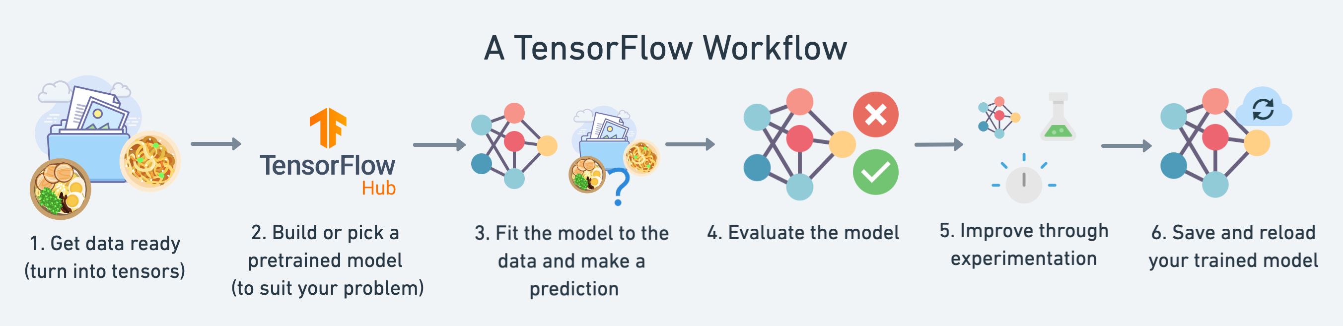 The workflow we're about to go through is a slightly modified version of the above image. As you keep going through deep learning problems, you'll find the workflow above is more of an outline than a step-by-step guide.
1. Import and become one with the data
Again, we've got a subset of the Food101 dataset. In addition to the pizza and steak images, we've pulled out another eight classes.
import zipfile
# Download zip file of 10_food_classes images
# See how this data was created - https://github.com/mrdbourke/tensorflow-deep-learning/blob/main/extras/image_data_modification.ipynb
!wget https://storage.googleapis.com/ztm_tf_course/food_vision/10_food_classes_all_data.zip
# Unzip the downloaded file
zip_ref = zipfile.ZipFile("10_food_classes_all_data.zip", "r")
zip_ref.extractall()
zip_ref.close()
--2023-05-11 04:00:59-- https://storage.googleapis.com/ztm_tf_course/food_vision/10_food_classes_all_data.zip Resolving storage.googleapis.com (storage.googleapis.com)... 108.177.127.128, 172.217.218.128, 142.250.153.128, ... Connecting to storage.googleapis.com (storage.googleapis.com)|108.177.127.128|:443... connected. HTTP request sent, awaiting response... 200 OK Length: 519183241 (495M) [application/zip] Saving to: ‘10_food_classes_all_data.zip’ 10_food_classes_all 100%[===================>] 495.13M 35.8MB/s in 15s 2023-05-11 04:01:15 (32.1 MB/s) - ‘10_food_classes_all_data.zip’ saved [519183241/519183241]
Now let's check out all of the different directories and sub-directories in the 10_food_classes file.
import os
# Walk through 10_food_classes directory and list number of files
for dirpath, dirnames, filenames in os.walk("10_food_classes_all_data"):
print(f"There are {len(dirnames)} directories and {len(filenames)} images in '{dirpath}'.")
There are 2 directories and 0 images in '10_food_classes_all_data'. There are 10 directories and 0 images in '10_food_classes_all_data/test'. There are 0 directories and 250 images in '10_food_classes_all_data/test/chicken_wings'. There are 0 directories and 250 images in '10_food_classes_all_data/test/fried_rice'. There are 0 directories and 250 images in '10_food_classes_all_data/test/ice_cream'. There are 0 directories and 250 images in '10_food_classes_all_data/test/grilled_salmon'. There are 0 directories and 250 images in '10_food_classes_all_data/test/chicken_curry'. There are 0 directories and 250 images in '10_food_classes_all_data/test/hamburger'. There are 0 directories and 250 images in '10_food_classes_all_data/test/steak'. There are 0 directories and 250 images in '10_food_classes_all_data/test/pizza'. There are 0 directories and 250 images in '10_food_classes_all_data/test/sushi'. There are 0 directories and 250 images in '10_food_classes_all_data/test/ramen'. There are 10 directories and 0 images in '10_food_classes_all_data/train'. There are 0 directories and 750 images in '10_food_classes_all_data/train/chicken_wings'. There are 0 directories and 750 images in '10_food_classes_all_data/train/fried_rice'. There are 0 directories and 750 images in '10_food_classes_all_data/train/ice_cream'. There are 0 directories and 750 images in '10_food_classes_all_data/train/grilled_salmon'. There are 0 directories and 750 images in '10_food_classes_all_data/train/chicken_curry'. There are 0 directories and 750 images in '10_food_classes_all_data/train/hamburger'. There are 0 directories and 750 images in '10_food_classes_all_data/train/steak'. There are 0 directories and 750 images in '10_food_classes_all_data/train/pizza'. There are 0 directories and 750 images in '10_food_classes_all_data/train/sushi'. There are 0 directories and 750 images in '10_food_classes_all_data/train/ramen'.
Looking good!
We'll now setup the training and test directory paths.
train_dir = "10_food_classes_all_data/train/"
test_dir = "10_food_classes_all_data/test/"
And get the class names from the subdirectories.
# Get the class names for our multi-class dataset
import pathlib
import numpy as np
data_dir = pathlib.Path(train_dir)
class_names = np.array(sorted([item.name for item in data_dir.glob('*')]))
print(class_names)
['chicken_curry' 'chicken_wings' 'fried_rice' 'grilled_salmon' 'hamburger' 'ice_cream' 'pizza' 'ramen' 'steak' 'sushi']
How about we visualize an image from the training set?
# View a random image from the training dataset
import random
img = view_random_image(target_dir=train_dir,
target_class=random.choice(class_names)) # get a random class name
Image shape: (512, 384, 3)

2. Preprocess the data (prepare it for a model)
After going through a handful of images (it's good to visualize at least 10-100 different examples), it looks like our data directories are setup correctly.
Time to preprocess the data.
from tensorflow.keras.preprocessing.image import ImageDataGenerator
# Rescale the data and create data generator instances
train_datagen = ImageDataGenerator(rescale=1/255.)
test_datagen = ImageDataGenerator(rescale=1/255.)
# Load data in from directories and turn it into batches
train_data = train_datagen.flow_from_directory(train_dir,
target_size=(224, 224),
batch_size=32,
class_mode='categorical') # changed to categorical
test_data = train_datagen.flow_from_directory(test_dir,
target_size=(224, 224),
batch_size=32,
class_mode='categorical')
Found 7500 images belonging to 10 classes. Found 2500 images belonging to 10 classes.
As with binary classifcation, we've creator image generators. The main change this time is that we've changed the class_mode parameter to 'categorical' because we're dealing with 10 classes of food images.
Everything else like rescaling the images, creating the batch size and target image size stay the same.
🤔 Question: Why is the image size 224x224? This could actually be any size we wanted, however, 224x224 is a very common size for preprocessing images to. Depending on your problem you might want to use larger or smaller images.
3. Create a model (start with a baseline)
We can use the same model (TinyVGG) we used for the binary classification problem for our multi-class classification problem with a couple of small tweaks.
Namely:
- Changing the output layer to use have 10 ouput neurons (the same number as the number of classes we have).
- Changing the output layer to use
'softmax'activation instead of'sigmoid'activation. - Changing the loss function to be
'categorical_crossentropy'instead of'binary_crossentropy'.
import tensorflow as tf
from tensorflow.keras.models import Sequential
from tensorflow.keras.layers import Conv2D, MaxPool2D, Flatten, Dense
# Create our model (a clone of model_8, except to be multi-class)
model_9 = Sequential([
Conv2D(10, 3, activation='relu', input_shape=(224, 224, 3)),
Conv2D(10, 3, activation='relu'),
MaxPool2D(),
Conv2D(10, 3, activation='relu'),
Conv2D(10, 3, activation='relu'),
MaxPool2D(),
Flatten(),
Dense(10, activation='softmax') # changed to have 10 neurons (same as number of classes) and 'softmax' activation
])
# Compile the model
model_9.compile(loss="categorical_crossentropy", # changed to categorical_crossentropy
optimizer=tf.keras.optimizers.Adam(),
metrics=["accuracy"])
4. Fit a model
Now we've got a model suited for working with multiple classes, let's fit it to our data.
# Fit the model
history_9 = model_9.fit(train_data, # now 10 different classes
epochs=5,
steps_per_epoch=len(train_data),
validation_data=test_data,
validation_steps=len(test_data))
Epoch 1/5 235/235 [==============================] - 48s 194ms/step - loss: 2.1520 - accuracy: 0.2133 - val_loss: 1.9674 - val_accuracy: 0.2964 Epoch 2/5 235/235 [==============================] - 45s 193ms/step - loss: 1.8770 - accuracy: 0.3489 - val_loss: 1.8792 - val_accuracy: 0.3424 Epoch 3/5 235/235 [==============================] - 45s 190ms/step - loss: 1.5239 - accuracy: 0.4860 - val_loss: 1.9865 - val_accuracy: 0.3184 Epoch 4/5 235/235 [==============================] - 45s 193ms/step - loss: 0.9507 - accuracy: 0.6897 - val_loss: 2.4049 - val_accuracy: 0.2824 Epoch 5/5 235/235 [==============================] - 45s 190ms/step - loss: 0.3835 - accuracy: 0.8772 - val_loss: 3.6373 - val_accuracy: 0.2760
Why do you think each epoch takes longer than when working with only two classes of images?
It's because we're now dealing with more images than we were before. We've got 10 classes with 750 training images and 250 validation images each totalling 10,000 images. Where as when we had two classes, we had 1500 training images and 500 validation images, totalling 2000.
The intuitive reasoning here is the more data you have, the longer a model will take to find patterns.
5. Evaluate the model
Woohoo! We've just trained a model on 10 different classes of food images, let's see how it went.
# Evaluate on the test data
model_9.evaluate(test_data)
79/79 [==============================] - 11s 139ms/step - loss: 3.6373 - accuracy: 0.2760
[3.6373109817504883, 0.2759999930858612]
# Check out the model's loss curves on the 10 classes of data (note: this function comes from above in the notebook)
plot_loss_curves(history_9)


Woah, that's quite the gap between the training and validation loss curves.
What does this tell us?
It seems our model is overfitting the training set quite badly. In other words, it's getting great results on the training data but fails to generalize well to unseen data and performs poorly on the test data.
6. Adjust the model parameters
Due to its performance on the training data, it's clear our model is learning something. However, performing well on the training data is like going well in the classroom but failing to use your skills in real life.
Ideally, we'd like our model to perform as well on the test data as it does on the training data.
So our next steps will be to try and prevent our model overfitting. A couple of ways to prevent overfitting include:
- Get more data - Having more data gives the model more opportunities to learn patterns, patterns which may be more generalizable to new examples.
- Simplify model - If the current model is already overfitting the training data, it may be too complicated of a model. This means it's learning the patterns of the data too well and isn't able to generalize well to unseen data. One way to simplify a model is to reduce the number of layers it uses or to reduce the number of hidden units in each layer.
- Use data augmentation - Data augmentation manipulates the training data in a way so that's harder for the model to learn as it artificially adds more variety to the data. If a model is able to learn patterns in augmented data, the model may be able to generalize better to unseen data.
- Use transfer learning - Transfer learning involves leverages the patterns (also called pretrained weights) one model has learned to use as the foundation for your own task. In our case, we could use one computer vision model pretrained on a large variety of images and then tweak it slightly to be more specialized for food images.
🔑 Note: Preventing overfitting is also referred to as regularization.
If you've already got an existing dataset, you're probably most likely to try one or a combination of the last three above options first.
Since collecting more data would involve us manually taking more images of food, let's try the ones we can do from right within the notebook.
How about we simplify our model first?
To do so, we'll remove two of the convolutional layers, taking the total number of convolutional layers from four to two.
# Try a simplified model (removed two layers)
model_10 = Sequential([
Conv2D(10, 3, activation='relu', input_shape=(224, 224, 3)),
MaxPool2D(),
Conv2D(10, 3, activation='relu'),
MaxPool2D(),
Flatten(),
Dense(10, activation='softmax')
])
model_10.compile(loss='categorical_crossentropy',
optimizer=tf.keras.optimizers.Adam(),
metrics=['accuracy'])
history_10 = model_10.fit(train_data,
epochs=5,
steps_per_epoch=len(train_data),
validation_data=test_data,
validation_steps=len(test_data))
Epoch 1/5 235/235 [==============================] - 46s 193ms/step - loss: 2.2804 - accuracy: 0.2397 - val_loss: 1.9445 - val_accuracy: 0.3024 Epoch 2/5 235/235 [==============================] - 45s 192ms/step - loss: 1.8253 - accuracy: 0.3785 - val_loss: 1.9529 - val_accuracy: 0.3172 Epoch 3/5 235/235 [==============================] - 44s 186ms/step - loss: 1.5193 - accuracy: 0.4979 - val_loss: 2.0705 - val_accuracy: 0.3160 Epoch 4/5 235/235 [==============================] - 44s 187ms/step - loss: 1.1143 - accuracy: 0.6408 - val_loss: 2.2653 - val_accuracy: 0.3064 Epoch 5/5 235/235 [==============================] - 44s 188ms/step - loss: 0.7340 - accuracy: 0.7787 - val_loss: 2.5814 - val_accuracy: 0.2944
# Check out the loss curves of model_10
plot_loss_curves(history_10)


Hmm... even with a simplifed model, it looks like our model is still dramatically overfitting the training data.
What else could we try?
How about data augmentation?
Data augmentation makes it harder for the model to learn on the training data and in turn, hopefully making the patterns it learns more generalizable to unseen data.
To create augmented data, we'll recreate a new ImageDataGenerator instance, this time adding some parameters such as rotation_range and horizontal_flip to manipulate our images.
# Create augmented data generator instance
train_datagen_augmented = ImageDataGenerator(rescale=1/255.,
rotation_range=20, # note: this is an int not a float
width_shift_range=0.2,
height_shift_range=0.2,
zoom_range=0.2,
horizontal_flip=True)
train_data_augmented = train_datagen_augmented.flow_from_directory(train_dir,
target_size=(224, 224),
batch_size=32,
class_mode='categorical')
Found 7500 images belonging to 10 classes.
Now we've got augmented data, let's see how it works with the same model as before (model_10).
Rather than rewrite the model from scratch, we can clone it using a handy function in TensorFlow called clone_model which can take an existing model and rebuild it in the same format.
The cloned version will not include any of the weights (patterns) the original model has learned. So when we train it, it'll be like training a model from scratch.
🔑 Note: One of the key practices in deep learning and machine learning in general is to be a serial experimenter. That's what we're doing here. Trying something, seeing if it works, then trying something else. A good experiment setup also keeps track of the things you change, for example, that's why we're using the same model as before but with different data. The model stays the same but the data changes, this will let us know if augmented training data has any influence over performance.
# Clone the model (use the same architecture)
model_11 = tf.keras.models.clone_model(model_10)
# Compile the cloned model (same setup as used for model_10)
model_11.compile(loss="categorical_crossentropy",
optimizer=tf.keras.optimizers.Adam(),
metrics=["accuracy"])
# Fit the model
history_11 = model_11.fit(train_data_augmented, # use augmented data
epochs=5,
steps_per_epoch=len(train_data_augmented),
validation_data=test_data,
validation_steps=len(test_data))
Epoch 1/5 235/235 [==============================] - 112s 473ms/step - loss: 2.1903 - accuracy: 0.1997 - val_loss: 2.0500 - val_accuracy: 0.2668 Epoch 2/5 235/235 [==============================] - 114s 483ms/step - loss: 2.0740 - accuracy: 0.2592 - val_loss: 1.9318 - val_accuracy: 0.3236 Epoch 3/5 235/235 [==============================] - 114s 485ms/step - loss: 2.0149 - accuracy: 0.3044 - val_loss: 1.8862 - val_accuracy: 0.3348 Epoch 4/5 235/235 [==============================] - 114s 487ms/step - loss: 1.9739 - accuracy: 0.3172 - val_loss: 1.8206 - val_accuracy: 0.3868 Epoch 5/5 235/235 [==============================] - 115s 489ms/step - loss: 1.9415 - accuracy: 0.3292 - val_loss: 1.8619 - val_accuracy: 0.3696
You can see it each epoch takes longer than the previous model. This is because our data is being augmented on the fly on the CPU as it gets loaded onto the GPU, in turn, increasing the amount of time between each epoch.
Note: One way to improve this time taken is to use augmentation layers directly as part of the model. For example, with
tf.keras.layers.RandomFlip. You can also speed up data loading with the newertf.keras.utils.image_dataset_from_directoryimage loading API (we cover this later in the course).
How do our model's training curves look?
# Check out our model's performance with augmented data
plot_loss_curves(history_11)


Woah! That's looking much better, the loss curves are much closer to eachother. Although our model didn't perform as well on the augmented training set, it performed much better on the validation dataset.
It even looks like if we kept it training for longer (more epochs) the evaluation metrics might continue to improve.
7. Repeat until satisfied
We could keep going here. Restructuring our model's architecture, adding more layers, trying it out, adjusting the learning rate, trying it out, trying different methods of data augmentation, training for longer. But as you could image, this could take a fairly long time.
Good thing there's still one trick we haven't tried yet and that's transfer learning.
However, we'll save that for the next notebook where you'll see how rather than design our own models from scratch we leverage the patterns another model has learned for our own task.
In the meantime, let's make a prediction with our trained multi-class model.
Making a prediction with our trained model
What good is a model if you can't make predictions with it?
Let's first remind ourselves of the classes our multi-class model has been trained on and then we'll download some of own custom images to work with.
# What classes has our model been trained on?
class_names
array(['chicken_curry', 'chicken_wings', 'fried_rice', 'grilled_salmon',
'hamburger', 'ice_cream', 'pizza', 'ramen', 'steak', 'sushi'],
dtype='<U14')
Beautiful, now let's get some of our custom images.
If you're using Google Colab, you could also upload some of your own images via the files tab.
# -q is for "quiet"
!wget -q https://raw.githubusercontent.com/mrdbourke/tensorflow-deep-learning/main/images/03-pizza-dad.jpeg
!wget -q https://raw.githubusercontent.com/mrdbourke/tensorflow-deep-learning/main/images/03-steak.jpeg
!wget -q https://raw.githubusercontent.com/mrdbourke/tensorflow-deep-learning/main/images/03-hamburger.jpeg
!wget -q https://raw.githubusercontent.com/mrdbourke/tensorflow-deep-learning/main/images/03-sushi.jpeg
Okay, we've got some custom images to try, let's use the pred_and_plot function to make a prediction with model_11 on one of the images and plot it.
# Make a prediction using model_11
pred_and_plot(model=model_11,
filename="03-steak.jpeg",
class_names=class_names)
1/1 [==============================] - 0s 81ms/step

Hmm... it looks like our model got the prediction wrong, how about we try another?
pred_and_plot(model_11, "03-sushi.jpeg", class_names)
1/1 [==============================] - 0s 23ms/step

And again, it's predicting chicken_curry for some reason.
How about one more?
pred_and_plot(model_11, "03-pizza-dad.jpeg", class_names)
1/1 [==============================] - 0s 22ms/step

chicken_curry again? There must be something wrong...
I think it might have to do with our pred_and_plot function.
Let's makes a prediction without using the function and see where it might be going wrong.
# Load in and preprocess our custom image
img = load_and_prep_image("03-steak.jpeg")
# Make a prediction
pred = model_11.predict(tf.expand_dims(img, axis=0))
# Match the prediction class to the highest prediction probability
pred_class = class_names[pred.argmax()]
plt.imshow(img)
plt.title(pred_class)
plt.axis(False);
1/1 [==============================] - 0s 22ms/step

Much better! There must be something up with our pred_and_plot function.
And I think I know what it is.
The pred_and_plot function was designed to be used with binary classification models where as our current model is a multi-class classification model.
The main difference lies in the output of the predict function.
# Check the output of the predict function
pred = model_11.predict(tf.expand_dims(img, axis=0))
pred
1/1 [==============================] - 0s 22ms/step
array([[0.00413127, 0.00698275, 0.00470221, 0.14550138, 0.0163848 ,
0.00341261, 0.00258247, 0.2162087 , 0.5952408 , 0.00485306]],
dtype=float32)
Since our model has a 'softmax' activation function and 10 output neurons, it outputs a prediction probability for each of the classes in our model.
The class with the highest probability is what the model believes the image contains.
We can find the maximum value index using argmax and then use that to index our class_names list to output the predicted class.
# Find the predicted class name
class_names[pred.argmax()]
'steak'
Knowing this, we can readjust our pred_and_plot function to work with multiple classes as well as binary classes.
# Adjust function to work with multi-class
def pred_and_plot(model, filename, class_names):
"""
Imports an image located at filename, makes a prediction on it with
a trained model and plots the image with the predicted class as the title.
"""
# Import the target image and preprocess it
img = load_and_prep_image(filename)
# Make a prediction
pred = model.predict(tf.expand_dims(img, axis=0))
# Get the predicted class
if len(pred[0]) > 1: # check for multi-class
pred_class = class_names[pred.argmax()] # if more than one output, take the max
else:
pred_class = class_names[int(tf.round(pred)[0][0])] # if only one output, round
# Plot the image and predicted class
plt.imshow(img)
plt.title(f"Prediction: {pred_class}")
plt.axis(False);
Let's try it out. If we've done it right, using different images should lead to different outputs (rather than chicken_curry every time).
pred_and_plot(model_11, "03-steak.jpeg", class_names)
1/1 [==============================] - 0s 23ms/step
pred_and_plot(model_11, "03-sushi.jpeg", class_names)
1/1 [==============================] - 0s 22ms/step

pred_and_plot(model_11, "03-pizza-dad.jpeg", class_names)
1/1 [==============================] - 0s 22ms/step

pred_and_plot(model_11, "03-hamburger.jpeg", class_names)
1/1 [==============================] - 0s 22ms/step

Our model's predictions aren't very good, this is because it's only performing at ~35% accuracy on the test dataset.
We'll see how to improve this later on (spolier: transfer learning is going to step things up a notch).
Saving and loading our model
Once you've trained a model, you probably want to be able to save it and load it somewhere else.
To do so, we can use the save and load_model functions.
# Save a model
model_11.save("saved_trained_model")
WARNING:absl:Found untraced functions such as _jit_compiled_convolution_op, _jit_compiled_convolution_op while saving (showing 2 of 2). These functions will not be directly callable after loading.
# Load in a model and evaluate it
loaded_model_11 = tf.keras.models.load_model("saved_trained_model")
loaded_model_11.evaluate(test_data)
79/79 [==============================] - 11s 141ms/step - loss: 1.8619 - accuracy: 0.3696
[1.8618727922439575, 0.36959999799728394]
# Compare our unsaved model's results (same as above)
model_11.evaluate(test_data)
79/79 [==============================] - 11s 140ms/step - loss: 1.8619 - accuracy: 0.3696
[1.8618724346160889, 0.36959999799728394]
🛠 Exercises
- Spend 20-minutes reading and interacting with the CNN explainer website.
- What are the key terms? e.g. explain convolution in your own words, pooling in your own words
- Play around with the "understanding hyperparameters" section in the CNN explainer website for 10-minutes.
- What is the kernel size?
- What is the stride?
- How could you adjust each of these in TensorFlow code?
Take 10 photos of two different things and build your own CNN image classifier using the techniques we've built here.
Find an ideal learning rate for a simple convolutional neural network model on your the 10 class dataset.
📖 Extra-curriculum
Watch: MIT's Introduction to Deep Computer Vision lecture. This will give you a great intuition behind convolutional neural networks.
Watch: Deep dive on mini-batch gradient descent by deeplearning.ai. If you're still curious about why we use batches to train models, this technical overview covers many of the reasons why.
Read: CS231n Convolutional Neural Networks for Visual Recognition class notes. This will give a very deep understanding of what's going on behind the scenes of the convolutional neural network architectures we're writing.
Read: "A guide to convolution arithmetic for deep learning". This paper goes through all of the mathematics running behind the scenes of our convolutional layers.
Code practice: TensorFlow Data Augmentation Tutorial. For a more in-depth introduction on data augmentation with TensorFlow, spend an hour or two reading through this tutorial.