![]()
09. Milestone Project 2: SkimLit 📄🔥
In the previous notebook (NLP fundamentals in TensorFlow), we went through some fundamental natural lanuage processing concepts. The main ones being tokenzation (turning words into numbers) and creating embeddings (creating a numerical representation of words).
In this project, we're going to be putting what we've learned into practice.
More specificially, we're going to be replicating the deep learning model behind the 2017 paper PubMed 200k RCT: a Dataset for Sequenctial Sentence Classification in Medical Abstracts.
When it was released, the paper presented a new dataset called PubMed 200k RCT which consists of ~200,000 labelled Randomized Controlled Trial (RCT) abstracts.
The goal of the dataset was to explore the ability for NLP models to classify sentences which appear in sequential order.
In other words, given the abstract of a RCT, what role does each sentence serve in the abstract?
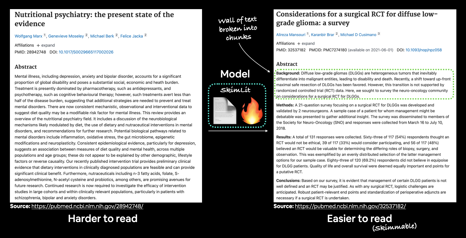
Example inputs (harder to read abstract from PubMed) and outputs (easier to read abstract) of the model we're going to build. The model will take an abstract wall of text and predict the section label each sentence should have.
Model Input
For example, can we train an NLP model which takes the following input (note: the following sample has had all numerical symbols replaced with "@"):
To investigate the efficacy of @ weeks of daily low-dose oral prednisolone in improving pain , mobility , and systemic low-grade inflammation in the short term and whether the effect would be sustained at @ weeks in older adults with moderate to severe knee osteoarthritis ( OA ). A total of @ patients with primary knee OA were randomized @:@ ; @ received @ mg/day of prednisolone and @ received placebo for @ weeks. Outcome measures included pain reduction and improvement in function scores and systemic inflammation markers. Pain was assessed using the visual analog pain scale ( @-@ mm ). Secondary outcome measures included the Western Ontario and McMaster Universities Osteoarthritis Index scores , patient global assessment ( PGA ) of the severity of knee OA , and @-min walk distance ( @MWD )., Serum levels of interleukin @ ( IL-@ ) , IL-@ , tumor necrosis factor ( TNF ) - , and high-sensitivity C-reactive protein ( hsCRP ) were measured. There was a clinically relevant reduction in the intervention group compared to the placebo group for knee pain , physical function , PGA , and @MWD at @ weeks. The mean difference between treatment arms ( @ % CI ) was @ ( @-@ @ ) , p < @ ; @ ( @-@ @ ) , p < @ ; @ ( @-@ @ ) , p < @ ; and @ ( @-@ @ ) , p < @ , respectively. Further , there was a clinically relevant reduction in the serum levels of IL-@ , IL-@ , TNF - , and hsCRP at @ weeks in the intervention group when compared to the placebo group. These differences remained significant at @ weeks. The Outcome Measures in Rheumatology Clinical Trials-Osteoarthritis Research Society International responder rate was @ % in the intervention group and @ % in the placebo group ( p < @ ). Low-dose oral prednisolone had both a short-term and a longer sustained effect resulting in less knee pain , better physical function , and attenuation of systemic inflammation in older patients with knee OA ( ClinicalTrials.gov identifier NCT@ ).
Model output
And returns the following output:
['###24293578\n',
 'OBJECTIVE\tTo investigate the efficacy of @ weeks of daily low-dose oral prednisolone in improving pain , mobility , and systemic low-grade inflammation in the short term and whether the effect would be sustained at @ weeks in older adults with moderate to severe knee osteoarthritis ( OA ) .\n',
 'METHODS\tA total of @ patients with primary knee OA were randomized @:@ ; @ received @ mg/day of prednisolone and @ received placebo for @ weeks .\n',
 'METHODS\tOutcome measures included pain reduction and improvement in function scores and systemic inflammation markers .\n',
 'METHODS\tPain was assessed using the visual analog pain scale ( @-@ mm ) .\n',
 'METHODS\tSecondary outcome measures included the Western Ontario and McMaster Universities Osteoarthritis Index scores , patient global assessment ( PGA ) of the severity of knee OA , and @-min walk distance ( @MWD ) .\n',
 'METHODS\tSerum levels of interleukin @ ( IL-@ ) , IL-@ , tumor necrosis factor ( TNF ) - , and high-sensitivity C-reactive protein ( hsCRP ) were measured .\n',
 'RESULTS\tThere was a clinically relevant reduction in the intervention group compared to the placebo group for knee pain , physical function , PGA , and @MWD at @ weeks .\n',
 'RESULTS\tThe mean difference between treatment arms ( @ % CI ) was @ ( @-@ @ ) , p < @ ; @ ( @-@ @ ) , p < @ ; @ ( @-@ @ ) , p < @ ; and @ ( @-@ @ ) , p < @ , respectively .\n',
 'RESULTS\tFurther , there was a clinically relevant reduction in the serum levels of IL-@ , IL-@ , TNF - , and hsCRP at @ weeks in the intervention group when compared to the placebo group .\n',
 'RESULTS\tThese differences remained significant at @ weeks .\n',
 'RESULTS\tThe Outcome Measures in Rheumatology Clinical Trials-Osteoarthritis Research Society International responder rate was @ % in the intervention group and @ % in the placebo group ( p < @ ) .\n',
 'CONCLUSIONS\tLow-dose oral prednisolone had both a short-term and a longer sustained effect resulting in less knee pain , better physical function , and attenuation of systemic inflammation in older patients with knee OA ( ClinicalTrials.gov identifier NCT@ ) .\n',
 '\n']
Problem in a sentence
The number of RCT papers released is continuing to increase, those without structured abstracts can be hard to read and in turn slow down researchers moving through the literature.
Solution in a sentence
Create an NLP model to classify abstract sentences into the role they play (e.g. objective, methods, results, etc) to enable researchers to skim through the literature (hence SkimLit 🤓🔥) and dive deeper when necessary.
- Where our data is coming from: PubMed 200k RCT: a Dataset for Sequential Sentence Classification in Medical Abstracts
- Where our model is coming from: Neural networks for joint sentence classification in medical paper abstracts.
📖 Resources: Before going through the code in this notebook, you might want to get a background of what we're going to be doing. To do so, spend an hour (or two) going through the following papers and then return to this notebook:
What we're going to cover
Time to take what we've learned in the NLP fundmentals notebook and build our biggest NLP model yet:
- Downloading a text dataset (PubMed RCT200k from GitHub)
- Writing a preprocessing function to prepare our data for modelling
- Setting up a series of modelling experiments
- Making a baseline (TF-IDF classifier)
- Deep models with different combinations of: token embeddings, character embeddings, pretrained embeddings, positional embeddings
- Building our first multimodal model (taking multiple types of data inputs)
- Replicating the model architecture from https://arxiv.org/abs/1612.05251
- Find the most wrong predictions
- Making predictions on PubMed abstracts from the wild
How you should approach this notebook
You can read through the descriptions and the code (it should all run, except for the cells which error on purpose), but there's a better option.
Write all of the code yourself.
Yes. I'm serious. Create a new notebook, and rewrite each line by yourself. Investigate it, see if you can break it, why does it break?
You don't have to write the text descriptions but writing the code yourself is a great way to get hands-on experience.
Don't worry if you make mistakes, we all do. The way to get better and make less mistakes is to write more code.
📖 Resources:
- See the full set of course materials on GitHub: https://github.com/mrdbourke/tensorflow-deep-learning
- See code updates to this notebook on GitHub discussions: https://github.com/mrdbourke/tensorflow-deep-learning/discussions/557
import datetime
print(f"Notebook last run (end-to-end): {datetime.datetime.now()}")
Notebook last run (end-to-end): 2023-05-26 03:47:27.469424
Confirm access to a GPU
Since we're going to be building deep learning models, let's make sure we have a GPU.
In Google Colab, you can set this up by going to Runtime -> Change runtime type -> Hardware accelerator -> GPU.
If you don't have access to a GPU, the models we're building here will likely take up to 10x longer to run.
# Check for GPU
!nvidia-smi -L
GPU 0: NVIDIA A100-SXM4-40GB (UUID: GPU-061bcc09-64a4-755a-357c-181dfae1f4a9)
Get data
Before we can start building a model, we've got to download the PubMed 200k RCT dataset.
In a phenomenal act of kindness, the authors of the paper have made the data they used for their research availably publically and for free in the form of .txt files on GitHub.
We can copy them to our local directory using git clone https://github.com/Franck-Dernoncourt/pubmed-rct.
!git clone https://github.com/Franck-Dernoncourt/pubmed-rct.git
!ls pubmed-rct
Cloning into 'pubmed-rct'...
remote: Enumerating objects: 33, done.
remote: Counting objects: 100% (8/8), done.
remote: Compressing objects: 100% (3/3), done.
remote: Total 33 (delta 5), reused 5 (delta 5), pack-reused 25
Unpacking objects: 100% (33/33), 177.08 MiB | 9.05 MiB/s, done.
PubMed_200k_RCT
PubMed_200k_RCT_numbers_replaced_with_at_sign
PubMed_20k_RCT
PubMed_20k_RCT_numbers_replaced_with_at_sign
README.md
Checking the contents of the downloaded repository, you can see there are four folders.
Each contains a different version of the PubMed 200k RCT dataset.
Looking at the README file from the GitHub page, we get the following information:
- PubMed 20k is a subset of PubMed 200k. I.e., any abstract present in PubMed 20k is also present in PubMed 200k.
PubMed_200k_RCTis the same asPubMed_200k_RCT_numbers_replaced_with_at_sign, except that in the latter all numbers had been replaced by@. (same forPubMed_20k_RCTvs.PubMed_20k_RCT_numbers_replaced_with_at_sign).- Since Github file size limit is 100 MiB, we had to compress
PubMed_200k_RCT\train.7zandPubMed_200k_RCT_numbers_replaced_with_at_sign\train.zip. To uncompresstrain.7z, you may use 7-Zip on Windows, Keka on Mac OS X, or p7zip on Linux.
To begin with, the dataset we're going to be focused on is PubMed_20k_RCT_numbers_replaced_with_at_sign.
Why this one?
Rather than working with the whole 200k dataset, we'll keep our experiments quick by starting with a smaller subset. We could've chosen the dataset with numbers instead of having them replaced with @ but we didn't.
Let's check the file contents.
# Check what files are in the PubMed_20K dataset
!ls pubmed-rct/PubMed_20k_RCT_numbers_replaced_with_at_sign
dev.txt test.txt train.txt
Beautiful, looks like we've got three separate text files:
train.txt- training samples.dev.txt- dev is short for development set, which is another name for validation set (in our case, we'll be using and referring to this file as our validation set).test.txt- test samples.
To save ourselves typing out the filepath to our target directory each time, let's turn it into a variable.
# Start by using the 20k dataset
data_dir = "pubmed-rct/PubMed_20k_RCT_numbers_replaced_with_at_sign/"
# Check all of the filenames in the target directory
import os
filenames = [data_dir + filename for filename in os.listdir(data_dir)]
filenames
['pubmed-rct/PubMed_20k_RCT_numbers_replaced_with_at_sign/test.txt',
 'pubmed-rct/PubMed_20k_RCT_numbers_replaced_with_at_sign/train.txt',
 'pubmed-rct/PubMed_20k_RCT_numbers_replaced_with_at_sign/dev.txt']
Preprocess data
Okay, now we've downloaded some text data, do you think we're ready to model it?
Wait...
We've downloaded the data but we haven't even looked at it yet.
What's the motto for getting familiar with any new dataset?
I'll give you a clue, the word begins with "v" and we say it three times.
Vibe, vibe, vibe?
Sort of... we've definitely got to the feel the vibe of our data.
Values, values, values?
Right again, we want to see lots of values but not quite what we're looking for.
Visualize, visualize, visualize?
Boom! That's it. To get familiar and understand how we have to prepare our data for our deep learning models, we've got to visualize it.
Because our data is in the form of text files, let's write some code to read each of the lines in a target file.
# Create function to read the lines of a document
def get_lines(filename):
  """
  Reads filename (a text file) and returns the lines of text as a list.

  Args:
      filename: a string containing the target filepath to read.

  Returns:
      A list of strings with one string per line from the target filename.
      For example:
      ["this is the first line of filename",
       "this is the second line of filename",
       "..."]
  """
  with open(filename, "r") as f:
    return f.readlines()
Alright, we've got a little function, get_lines() which takes the filepath of a text file, opens it, reads each of the lines and returns them.
Let's try it out on the training data (train.txt).
train_lines = get_lines(data_dir+"train.txt")
train_lines[:20] # the whole first example of an abstract + a little more of the next one
['###24293578\n',
 'OBJECTIVE\tTo investigate the efficacy of @ weeks of daily low-dose oral prednisolone in improving pain , mobility , and systemic low-grade inflammation in the short term and whether the effect would be sustained at @ weeks in older adults with moderate to severe knee osteoarthritis ( OA ) .\n',
 'METHODS\tA total of @ patients with primary knee OA were randomized @:@ ; @ received @ mg/day of prednisolone and @ received placebo for @ weeks .\n',
 'METHODS\tOutcome measures included pain reduction and improvement in function scores and systemic inflammation markers .\n',
 'METHODS\tPain was assessed using the visual analog pain scale ( @-@ mm ) .\n',
 'METHODS\tSecondary outcome measures included the Western Ontario and McMaster Universities Osteoarthritis Index scores , patient global assessment ( PGA ) of the severity of knee OA , and @-min walk distance ( @MWD ) .\n',
 'METHODS\tSerum levels of interleukin @ ( IL-@ ) , IL-@ , tumor necrosis factor ( TNF ) - , and high-sensitivity C-reactive protein ( hsCRP ) were measured .\n',
 'RESULTS\tThere was a clinically relevant reduction in the intervention group compared to the placebo group for knee pain , physical function , PGA , and @MWD at @ weeks .\n',
 'RESULTS\tThe mean difference between treatment arms ( @ % CI ) was @ ( @-@ @ ) , p < @ ; @ ( @-@ @ ) , p < @ ; @ ( @-@ @ ) , p < @ ; and @ ( @-@ @ ) , p < @ , respectively .\n',
 'RESULTS\tFurther , there was a clinically relevant reduction in the serum levels of IL-@ , IL-@ , TNF - , and hsCRP at @ weeks in the intervention group when compared to the placebo group .\n',
 'RESULTS\tThese differences remained significant at @ weeks .\n',
 'RESULTS\tThe Outcome Measures in Rheumatology Clinical Trials-Osteoarthritis Research Society International responder rate was @ % in the intervention group and @ % in the placebo group ( p < @ ) .\n',
 'CONCLUSIONS\tLow-dose oral prednisolone had both a short-term and a longer sustained effect resulting in less knee pain , better physical function , and attenuation of systemic inflammation in older patients with knee OA ( ClinicalTrials.gov identifier NCT@ ) .\n',
 '\n',
 '###24854809\n',
 'BACKGROUND\tEmotional eating is associated with overeating and the development of obesity .\n',
 'BACKGROUND\tYet , empirical evidence for individual ( trait ) differences in emotional eating and cognitive mechanisms that contribute to eating during sad mood remain equivocal .\n',
 'OBJECTIVE\tThe aim of this study was to test if attention bias for food moderates the effect of self-reported emotional eating during sad mood ( vs neutral mood ) on actual food intake .\n',
 'OBJECTIVE\tIt was expected that emotional eating is predictive of elevated attention for food and higher food intake after an experimentally induced sad mood and that attentional maintenance on food predicts food intake during a sad versus a neutral mood .\n',
 'METHODS\tParticipants ( N = @ ) were randomly assigned to one of the two experimental mood induction conditions ( sad/neutral ) .\n']
Reading the lines from the training text file results in a list of strings containing different abstract samples, the sentences in a sample along with the role the sentence plays in the abstract.
The role of each sentence is prefixed at the start of each line separated by a tab (\t) and each sentence finishes with a new line (\n).
Different abstracts are separated by abstract ID's (lines beginning with ###) and newlines (\n).
Knowing this, it looks like we've got a couple of steps to do to get our samples ready to pass as training data to our future machine learning model.
Let's write a function to perform the following steps:
- Take a target file of abstract samples.
- Read the lines in the target file.
- For each line in the target file:
- If the line begins with
###mark it as an abstract ID and the beginning of a new abstract.- Keep count of the number of lines in a sample.
- If the line begins with
\nmark it as the end of an abstract sample.- Keep count of the total lines in a sample.
- Record the text before the
\tas the label of the line. - Record the text after the
\tas the text of the line.
- If the line begins with
- Return all of the lines in the target text file as a list of dictionaries containing the key/value pairs:
"line_number"- the position of the line in the abstract (e.g.3)."target"- the role of the line in the abstract (e.g.OBJECTIVE)."text"- the text of the line in the abstract."total_lines"- the total lines in an abstract sample (e.g.14).
- Abstract ID's and newlines should be omitted from the returned preprocessed data.
Example returned preprocessed sample (a single line from an abstract):
[{'line_number': 0,
  'target': 'OBJECTIVE',
  'text': 'to investigate the efficacy of @ weeks of daily low-dose oral prednisolone in improving pain , mobility , and systemic low-grade inflammation in the short term and whether the effect would be sustained at @ weeks in older adults with moderate to severe knee osteoarthritis ( oa ) .',
  'total_lines': 11},
  ...]
def preprocess_text_with_line_numbers(filename):
  """Returns a list of dictionaries of abstract line data.

  Takes in filename, reads its contents and sorts through each line,
  extracting things like the target label, the text of the sentence,
  how many sentences are in the current abstract and what sentence number
  the target line is.

  Args:
      filename: a string of the target text file to read and extract line data
      from.

  Returns:
      A list of dictionaries each containing a line from an abstract,
      the lines label, the lines position in the abstract and the total number
      of lines in the abstract where the line is from. For example:

      [{"target": 'CONCLUSION',
        "text": The study couldn't have gone better, turns out people are kinder than you think",
        "line_number": 8,
        "total_lines": 8}]
  """
  input_lines = get_lines(filename) # get all lines from filename
  abstract_lines = "" # create an empty abstract
  abstract_samples = [] # create an empty list of abstracts

  # Loop through each line in target file
  for line in input_lines:
    if line.startswith("###"): # check to see if line is an ID line
      abstract_id = line
      abstract_lines = "" # reset abstract string
    elif line.isspace(): # check to see if line is a new line
      abstract_line_split = abstract_lines.splitlines() # split abstract into separate lines

      # Iterate through each line in abstract and count them at the same time
      for abstract_line_number, abstract_line in enumerate(abstract_line_split):
        line_data = {} # create empty dict to store data from line
        target_text_split = abstract_line.split("\t") # split target label from text
        line_data["target"] = target_text_split[0] # get target label
        line_data["text"] = target_text_split[1].lower() # get target text and lower it
        line_data["line_number"] = abstract_line_number # what number line does the line appear in the abstract?
        line_data["total_lines"] = len(abstract_line_split) - 1 # how many total lines are in the abstract? (start from 0)
        abstract_samples.append(line_data) # add line data to abstract samples list

    else: # if the above conditions aren't fulfilled, the line contains a labelled sentence
      abstract_lines += line

  return abstract_samples
Beautiful! That's one good looking function. Let's use it to preprocess each of our RCT 20k datasets.
# Get data from file and preprocess it
%%time
train_samples = preprocess_text_with_line_numbers(data_dir + "train.txt")
val_samples = preprocess_text_with_line_numbers(data_dir + "dev.txt") # dev is another name for validation set
test_samples = preprocess_text_with_line_numbers(data_dir + "test.txt")
len(train_samples), len(val_samples), len(test_samples)
CPU times: user 344 ms, sys: 77.2 ms, total: 421 ms
Wall time: 420 ms
(180040, 30212, 30135)
How do our training samples look?
# Check the first abstract of our training data
train_samples[:14]
[{'target': 'OBJECTIVE',
  'text': 'to investigate the efficacy of @ weeks of daily low-dose oral prednisolone in improving pain , mobility , and systemic low-grade inflammation in the short term and whether the effect would be sustained at @ weeks in older adults with moderate to severe knee osteoarthritis ( oa ) .',
  'line_number': 0,
  'total_lines': 11},
 {'target': 'METHODS',
  'text': 'a total of @ patients with primary knee oa were randomized @:@ ; @ received @ mg/day of prednisolone and @ received placebo for @ weeks .',
  'line_number': 1,
  'total_lines': 11},
 {'target': 'METHODS',
  'text': 'outcome measures included pain reduction and improvement in function scores and systemic inflammation markers .',
  'line_number': 2,
  'total_lines': 11},
 {'target': 'METHODS',
  'text': 'pain was assessed using the visual analog pain scale ( @-@ mm ) .',
  'line_number': 3,
  'total_lines': 11},
 {'target': 'METHODS',
  'text': 'secondary outcome measures included the western ontario and mcmaster universities osteoarthritis index scores , patient global assessment ( pga ) of the severity of knee oa , and @-min walk distance ( @mwd ) .',
  'line_number': 4,
  'total_lines': 11},
 {'target': 'METHODS',
  'text': 'serum levels of interleukin @ ( il-@ ) , il-@ , tumor necrosis factor ( tnf ) - , and high-sensitivity c-reactive protein ( hscrp ) were measured .',
  'line_number': 5,
  'total_lines': 11},
 {'target': 'RESULTS',
  'text': 'there was a clinically relevant reduction in the intervention group compared to the placebo group for knee pain , physical function , pga , and @mwd at @ weeks .',
  'line_number': 6,
  'total_lines': 11},
 {'target': 'RESULTS',
  'text': 'the mean difference between treatment arms ( @ % ci ) was @ ( @-@ @ ) , p < @ ; @ ( @-@ @ ) , p < @ ; @ ( @-@ @ ) , p < @ ; and @ ( @-@ @ ) , p < @ , respectively .',
  'line_number': 7,
  'total_lines': 11},
 {'target': 'RESULTS',
  'text': 'further , there was a clinically relevant reduction in the serum levels of il-@ , il-@ , tnf - , and hscrp at @ weeks in the intervention group when compared to the placebo group .',
  'line_number': 8,
  'total_lines': 11},
 {'target': 'RESULTS',
  'text': 'these differences remained significant at @ weeks .',
  'line_number': 9,
  'total_lines': 11},
 {'target': 'RESULTS',
  'text': 'the outcome measures in rheumatology clinical trials-osteoarthritis research society international responder rate was @ % in the intervention group and @ % in the placebo group ( p < @ ) .',
  'line_number': 10,
  'total_lines': 11},
 {'target': 'CONCLUSIONS',
  'text': 'low-dose oral prednisolone had both a short-term and a longer sustained effect resulting in less knee pain , better physical function , and attenuation of systemic inflammation in older patients with knee oa ( clinicaltrials.gov identifier nct@ ) .',
  'line_number': 11,
  'total_lines': 11},
 {'target': 'BACKGROUND',
  'text': 'emotional eating is associated with overeating and the development of obesity .',
  'line_number': 0,
  'total_lines': 10},
 {'target': 'BACKGROUND',
  'text': 'yet , empirical evidence for individual ( trait ) differences in emotional eating and cognitive mechanisms that contribute to eating during sad mood remain equivocal .',
  'line_number': 1,
  'total_lines': 10}]
Fantastic! Looks like our preprocess_text_with_line_numbers() function worked great.
How about we turn our list of dictionaries into pandas DataFrame's so we visualize them better?
import pandas as pd
train_df = pd.DataFrame(train_samples)
val_df = pd.DataFrame(val_samples)
test_df = pd.DataFrame(test_samples)
train_df.head(14)
| target | text | line_number | total_lines | |
|---|---|---|---|---|
| 0 | OBJECTIVE | to investigate the efficacy of @ weeks of dail... | 0 | 11 |
| 1 | METHODS | a total of @ patients with primary knee oa wer... | 1 | 11 |
| 2 | METHODS | outcome measures included pain reduction and i... | 2 | 11 |
| 3 | METHODS | pain was assessed using the visual analog pain... | 3 | 11 |
| 4 | METHODS | secondary outcome measures included the wester... | 4 | 11 |
| 5 | METHODS | serum levels of interleukin @ ( il-@ ) , il-@ ... | 5 | 11 |
| 6 | RESULTS | there was a clinically relevant reduction in t... | 6 | 11 |
| 7 | RESULTS | the mean difference between treatment arms ( @... | 7 | 11 |
| 8 | RESULTS | further , there was a clinically relevant redu... | 8 | 11 |
| 9 | RESULTS | these differences remained significant at @ we... | 9 | 11 |
| 10 | RESULTS | the outcome measures in rheumatology clinical ... | 10 | 11 |
| 11 | CONCLUSIONS | low-dose oral prednisolone had both a short-te... | 11 | 11 |
| 12 | BACKGROUND | emotional eating is associated with overeating... | 0 | 10 |
| 13 | BACKGROUND | yet , empirical evidence for individual ( trai... | 1 | 10 |
Now our data is in DataFrame form, we can perform some data analysis on it.
# Distribution of labels in training data
train_df.target.value_counts()
METHODS        59353
RESULTS        57953
CONCLUSIONS    27168
BACKGROUND     21727
OBJECTIVE      13839
Name: target, dtype: int64
Looks like sentences with the OBJECTIVE label are the least common.
How about we check the distribution of our abstract lengths?
train_df.total_lines.plot.hist();

Okay, looks like most of the abstracts are around 7 to 15 sentences in length.
It's good to check these things out to make sure when we do train a model or test it on unseen samples, our results aren't outlandish.
Get lists of sentences
When we build our deep learning model, one of its main inputs will be a list of strings (the lines of an abstract).
We can get these easily from our DataFrames by calling the tolist() method on our "text" columns.
# Convert abstract text lines into lists
train_sentences = train_df["text"].tolist()
val_sentences = val_df["text"].tolist()
test_sentences = test_df["text"].tolist()
len(train_sentences), len(val_sentences), len(test_sentences)
(180040, 30212, 30135)
# View first 10 lines of training sentences
train_sentences[:10]
['to investigate the efficacy of @ weeks of daily low-dose oral prednisolone in improving pain , mobility , and systemic low-grade inflammation in the short term and whether the effect would be sustained at @ weeks in older adults with moderate to severe knee osteoarthritis ( oa ) .',
 'a total of @ patients with primary knee oa were randomized @:@ ; @ received @ mg/day of prednisolone and @ received placebo for @ weeks .',
 'outcome measures included pain reduction and improvement in function scores and systemic inflammation markers .',
 'pain was assessed using the visual analog pain scale ( @-@ mm ) .',
 'secondary outcome measures included the western ontario and mcmaster universities osteoarthritis index scores , patient global assessment ( pga ) of the severity of knee oa , and @-min walk distance ( @mwd ) .',
 'serum levels of interleukin @ ( il-@ ) , il-@ , tumor necrosis factor ( tnf ) - , and high-sensitivity c-reactive protein ( hscrp ) were measured .',
 'there was a clinically relevant reduction in the intervention group compared to the placebo group for knee pain , physical function , pga , and @mwd at @ weeks .',
 'the mean difference between treatment arms ( @ % ci ) was @ ( @-@ @ ) , p < @ ; @ ( @-@ @ ) , p < @ ; @ ( @-@ @ ) , p < @ ; and @ ( @-@ @ ) , p < @ , respectively .',
 'further , there was a clinically relevant reduction in the serum levels of il-@ , il-@ , tnf - , and hscrp at @ weeks in the intervention group when compared to the placebo group .',
 'these differences remained significant at @ weeks .']
Alright, we've separated our text samples. As you might've guessed, we'll have to write code to convert the text to numbers before we can use it with our machine learning models, we'll get to this soon.
Make numeric labels (ML models require numeric labels)
We're going to create one hot and label encoded labels.
We could get away with just making label encoded labels, however, TensorFlow's CategoricalCrossentropy loss function likes to have one hot encoded labels (this will enable us to use label smoothing later on).
To numerically encode labels we'll use Scikit-Learn's OneHotEncoder and LabelEncoder classes.
# One hot encode labels
from sklearn.preprocessing import OneHotEncoder
one_hot_encoder = OneHotEncoder(sparse=False)
train_labels_one_hot = one_hot_encoder.fit_transform(train_df["target"].to_numpy().reshape(-1, 1))
val_labels_one_hot = one_hot_encoder.transform(val_df["target"].to_numpy().reshape(-1, 1))
test_labels_one_hot = one_hot_encoder.transform(test_df["target"].to_numpy().reshape(-1, 1))

# Check what training labels look like
train_labels_one_hot
/usr/local/lib/python3.10/dist-packages/sklearn/preprocessing/_encoders.py:868: FutureWarning: `sparse` was renamed to `sparse_output` in version 1.2 and will be removed in 1.4. `sparse_output` is ignored unless you leave `sparse` to its default value.
  warnings.warn(
array([[0., 0., 0., 1., 0.],
       [0., 0., 1., 0., 0.],
       [0., 0., 1., 0., 0.],
       ...,
       [0., 0., 0., 0., 1.],
       [0., 1., 0., 0., 0.],
       [0., 1., 0., 0., 0.]])
Label encode labels
# Extract labels ("target" columns) and encode them into integers
from sklearn.preprocessing import LabelEncoder
label_encoder = LabelEncoder()
train_labels_encoded = label_encoder.fit_transform(train_df["target"].to_numpy())
val_labels_encoded = label_encoder.transform(val_df["target"].to_numpy())
test_labels_encoded = label_encoder.transform(test_df["target"].to_numpy())

# Check what training labels look like
train_labels_encoded
array([3, 2, 2, ..., 4, 1, 1])
Now we've trained an instance of LabelEncoder, we can get the class names and number of classes using the classes_ attribute.
# Get class names and number of classes from LabelEncoder instance
num_classes = len(label_encoder.classes_)
class_names = label_encoder.classes_
num_classes, class_names
(5,
 array(['BACKGROUND', 'CONCLUSIONS', 'METHODS', 'OBJECTIVE', 'RESULTS'],
       dtype=object))
Creating a series of model experiments
We've proprocessed our data so now, in true machine learning fashion, it's time to setup a series of modelling experiments.
We'll start by creating a simple baseline model to obtain a score we'll try to beat by building more and more complex models as we move towards replicating the sequence model outlined in Neural networks for joint sentence classification in medical paper abstracts.
For each model, we'll train it on the training data and evaluate it on the validation data.
Model 0: Getting a baseline
Our first model we'll be a TF-IDF Multinomial Naive Bayes as recommended by Scikit-Learn's machine learning map.
To build it, we'll create a Scikit-Learn Pipeline which uses the TfidfVectorizer class to convert our abstract sentences to numbers using the TF-IDF (term frequency-inverse document frequecy) algorithm and then learns to classify our sentences using the MultinomialNB aglorithm.
from sklearn.feature_extraction.text import TfidfVectorizer
from sklearn.naive_bayes import MultinomialNB
from sklearn.pipeline import Pipeline

# Create a pipeline
model_0 = Pipeline([
  ("tf-idf", TfidfVectorizer()),
  ("clf", MultinomialNB())
])

# Fit the pipeline to the training data
model_0.fit(X=train_sentences,
            y=train_labels_encoded);
Due to the speed of the Multinomial Naive Bayes algorithm, it trains very quickly.
We can evaluate our model's accuracy on the validation dataset using the score() method.
# Evaluate baseline on validation dataset
model_0.score(X=val_sentences,
              y=val_labels_encoded)
0.7218323844829869
Nice! Looks like 72.1% accuracy will be the number to beat with our deeper models.
Now let's make some predictions with our baseline model to further evaluate it.
# Make predictions
baseline_preds = model_0.predict(val_sentences)
baseline_preds
array([4, 1, 3, ..., 4, 4, 1])
To evaluate our baseline's predictions, we'll import the calculate_results() function we created in the previous notebook and added it to our helper_functions.py script to compare them to the ground truth labels.
More specificially the calculate_results() function will help us obtain the following:
- Accuracy
- Precision
- Recall
- F1-score
Download helper functions script
Let's get our helper_functions.py script we've been using to store helper functions we've created in previous notebooks.
# Download helper functions script
!wget https://raw.githubusercontent.com/mrdbourke/tensorflow-deep-learning/main/extras/helper_functions.py
--2023-05-26 03:47:55--  https://raw.githubusercontent.com/mrdbourke/tensorflow-deep-learning/main/extras/helper_functions.py
Resolving raw.githubusercontent.com (raw.githubusercontent.com)... 185.199.108.133, 185.199.109.133, 185.199.110.133, ...
Connecting to raw.githubusercontent.com (raw.githubusercontent.com)|185.199.108.133|:443... connected.
HTTP request sent, awaiting response... 200 OK
Length: 10246 (10K) [text/plain]
Saving to: ‘helper_functions.py’


helper_functions.py   0%[                    ]       0  --.-KB/s
helper_functions.py 100%[===================>]  10.01K  --.-KB/s    in 0s

2023-05-26 03:47:55 (118 MB/s) - ‘helper_functions.py’ saved [10246/10246]
Now we've got the helper functions script we can import the caculate_results() function and see how our baseline model went.
# Import calculate_results helper function
from helper_functions import calculate_results
# Calculate baseline results
baseline_results = calculate_results(y_true=val_labels_encoded,
                                     y_pred=baseline_preds)
baseline_results
{'accuracy': 72.1832384482987,
 'precision': 0.7186466952323352,
 'recall': 0.7218323844829869,
 'f1': 0.6989250353450294}
Preparing our data for deep sequence models
Excellent! We've got a working baseline to try and improve upon.
But before we start building deeper models, we've got to create vectorization and embedding layers.
The vectorization layer will convert our text to numbers and the embedding layer will capture the relationships between those numbers.
To start creating our vectorization and embedding layers, we'll need to import the appropriate libraries (namely TensorFlow and NumPy).
import numpy as np
import tensorflow as tf
from tensorflow.keras import layers
Since we'll be turning our sentences into numbers, it's a good idea to figure out how many words are in each sentence.
When our model goes through our sentences, it works best when they're all the same length (this is important for creating batches of the same size tensors).
For example, if one sentence is eight words long and another is 29 words long, we want to pad the eight word sentence with zeros so it ends up being the same length as the 29 word sentence.
Let's write some code to find the average length of sentences in the training set.
# How long is each sentence on average?
sent_lens = [len(sentence.split()) for sentence in train_sentences]
avg_sent_len = np.mean(sent_lens)
avg_sent_len # return average sentence length (in tokens)
26.338269273494777
How about the distribution of sentence lengths?
# What's the distribution look like?
import matplotlib.pyplot as plt
plt.hist(sent_lens, bins=7);

Looks like the vast majority of sentences are between 0 and 50 tokens in length.
We can use NumPy's percentile to find the value which covers 95% of the sentence lengths.
# How long of a sentence covers 95% of the lengths?
output_seq_len = int(np.percentile(sent_lens, 95))
output_seq_len
55
Wonderful! It looks like 95% of the sentences in our training set have a length of 55 tokens or less.
When we create our tokenization layer, we'll use this value to turn all of our sentences into the same length. Meaning sentences with a length below 55 get padded with zeros and sentences with a length above 55 get truncated (words after 55 get cut off).
🤔 Question: Why 95%?
We could use the max sentence length of the sentences in the training set.
# Maximum sentence length in the training set
max(sent_lens)
296
However, since hardly any sentences even come close to the max length, it would mean the majority of the data we pass to our model would be zeros (sinces all sentences below the max length would get padded with zeros).
🔑 Note: The steps we've gone through are good practice when working with a text corpus for a NLP problem. You want to know how long your samples are and what the distribution of them is. See section 4 Data Analysis of the PubMed 200k RCT paper for further examples.
Create text vectorizer
Now we've got a little more information about our texts, let's create a way to turn it into numbers.
To do so, we'll use the TextVectorization layer from TensorFlow.
We'll keep all the parameters default except for max_tokens (the number of unique words in our dataset) and output_sequence_length (our desired output length for each vectorized sentence).
Section 3.2 of the PubMed 200k RCT paper states the vocabulary size of the PubMed 20k dataset as 68,000. So we'll use that as our max_tokens parameter.
# How many words are in our vocabulary? (taken from 3.2 in https://arxiv.org/pdf/1710.06071.pdf)
max_tokens = 68000
And since discovered a sentence length of 55 covers 95% of the training sentences, we'll use that as our output_sequence_length parameter.
# Create text vectorizer

# After TensorFlow 2.6
from tensorflow.keras.layers import TextVectorization

# Before TensorFlow 2.6
# from tensorflow.keras.layers.experimental.preprocessing import TextVectorization

text_vectorizer = TextVectorization(max_tokens=max_tokens, # number of words in vocabulary
                                    output_sequence_length=55) # desired output length of vectorized sequences
Great! Looks like our text_vectorizer is ready, let's adapt it to the training data (let it read the training data and figure out what number should represent what word) and then test it out.
# Adapt text vectorizer to training sentences
text_vectorizer.adapt(train_sentences)
# Test out text vectorizer
import random
target_sentence = random.choice(train_sentences)
print(f"Text:\n{target_sentence}")
print(f"\nLength of text: {len(target_sentence.split())}")
print(f"\nVectorized text:\n{text_vectorizer([target_sentence])}")
Text:
patients later completed a ten-question true-or-false knowledge questionnaire and a six-item satisfaction survey .

Length of text: 14

Vectorized text:
[[   12   869   253     8 44042 43177   494   325     3     8 34340   428
    885     0     0     0     0     0     0     0     0     0     0     0
      0     0     0     0     0     0     0     0     0     0     0     0
      0     0     0     0     0     0     0     0     0     0     0     0
      0     0     0     0     0     0     0]]
Cool, we've now got a way to turn our sequences into numbers.
🛠 Exercise: Try running the cell above a dozen or so times. What do you notice about sequences with a length less than 55?
Using the get_vocabulary() method of our text_vectorizer we can find out a few different tidbits about our text.
# How many words in our training vocabulary?
rct_20k_text_vocab = text_vectorizer.get_vocabulary()
print(f"Number of words in vocabulary: {len(rct_20k_text_vocab)}"),
print(f"Most common words in the vocabulary: {rct_20k_text_vocab[:5]}")
print(f"Least common words in the vocabulary: {rct_20k_text_vocab[-5:]}")
Number of words in vocabulary: 64841
Most common words in the vocabulary: ['', '[UNK]', 'the', 'and', 'of']
Least common words in the vocabulary: ['aainduced', 'aaigroup', 'aachener', 'aachen', 'aaacp']
And if we wanted to figure out the configuration of our text_vectorizer we can use the get_config() method.
# Get the config of our text vectorizer
text_vectorizer.get_config()
{'name': 'text_vectorization',
 'trainable': True,
 'dtype': 'string',
 'batch_input_shape': (None,),
 'max_tokens': 68000,
 'standardize': 'lower_and_strip_punctuation',
 'split': 'whitespace',
 'ngrams': None,
 'output_mode': 'int',
 'output_sequence_length': 55,
 'pad_to_max_tokens': False,
 'sparse': False,
 'ragged': False,
 'vocabulary': None,
 'idf_weights': None,
 'encoding': 'utf-8',
 'vocabulary_size': 64841}
Create custom text embedding
Our token_vectorization layer maps the words in our text directly to numbers. However, this doesn't necessarily capture the relationships between those numbers.
To create a richer numerical representation of our text, we can use an embedding.
As our model learns (by going through many different examples of abstract sentences and their labels), it'll update its embedding to better represent the relationships between tokens in our corpus.
We can create a trainable embedding layer using TensorFlow's Embedding layer.
Once again, the main parameters we're concerned with here are the inputs and outputs of our Embedding layer.
The input_dim parameter defines the size of our vocabulary. And the output_dim parameter defines the dimension of the embedding output.
Once created, our embedding layer will take the integer outputs of our text_vectorization layer as inputs and convert them to feature vectors of size output_dim.
Let's see it in action.
# Create token embedding layer
token_embed = layers.Embedding(input_dim=len(rct_20k_text_vocab), # length of vocabulary
                               output_dim=128, # Note: different embedding sizes result in drastically different numbers of parameters to train
                               # Use masking to handle variable sequence lengths (save space)
                               mask_zero=True,
                               name="token_embedding")

# Show example embedding
print(f"Sentence before vectorization:\n{target_sentence}\n")
vectorized_sentence = text_vectorizer([target_sentence])
print(f"Sentence after vectorization (before embedding):\n{vectorized_sentence}\n")
embedded_sentence = token_embed(vectorized_sentence)
print(f"Sentence after embedding:\n{embedded_sentence}\n")
print(f"Embedded sentence shape: {embedded_sentence.shape}")
Sentence before vectorization:
patients later completed a ten-question true-or-false knowledge questionnaire and a six-item satisfaction survey .

Sentence after vectorization (before embedding):
[[   12   869   253     8 44042 43177   494   325     3     8 34340   428
    885     0     0     0     0     0     0     0     0     0     0     0
      0     0     0     0     0     0     0     0     0     0     0     0
      0     0     0     0     0     0     0     0     0     0     0     0
      0     0     0     0     0     0     0]]

Sentence after embedding:
[[[ 0.03009653 -0.00744227  0.03255219 ...  0.04350514  0.02615802
    0.01004974]
  [ 0.00894579 -0.04471136  0.04325384 ...  0.00689     0.03921053
   -0.01831497]
  [ 0.0371519   0.01963044 -0.0322178  ...  0.01794907 -0.00109234
    0.02466574]
  ...
  [ 0.03691586 -0.00786442 -0.04396362 ...  0.04501832  0.00408162
   -0.02123723]
  [ 0.03691586 -0.00786442 -0.04396362 ...  0.04501832  0.00408162
   -0.02123723]
  [ 0.03691586 -0.00786442 -0.04396362 ...  0.04501832  0.00408162
   -0.02123723]]]

Embedded sentence shape: (1, 55, 128)
Create datasets (as fast as possible)
We've gone through all the trouble of preprocessing our datasets to be used with a machine learning model, however, there are still a few steps we can use to make them work faster with our models.
Namely, the tf.data API provides methods which enable faster data loading.
📖 Resource: For best practices on data loading in TensorFlow, check out the following:
The main steps we'll want to use with our data is to turn it into a PrefetchDataset of batches.
Doing so we'll ensure TensorFlow loads our data onto the GPU as fast as possible, in turn leading to faster training time.
To create a batched PrefetchDataset we can use the methods batch() and prefetch(), the parameter tf.data.AUTOTUNE will also allow TensorFlow to determine the optimal amount of compute to use to prepare datasets.
# Turn our data into TensorFlow Datasets
train_dataset = tf.data.Dataset.from_tensor_slices((train_sentences, train_labels_one_hot))
valid_dataset = tf.data.Dataset.from_tensor_slices((val_sentences, val_labels_one_hot))
test_dataset = tf.data.Dataset.from_tensor_slices((test_sentences, test_labels_one_hot))

train_dataset
<_TensorSliceDataset element_spec=(TensorSpec(shape=(), dtype=tf.string, name=None), TensorSpec(shape=(5,), dtype=tf.float64, name=None))>
# Take the TensorSliceDataset's and turn them into prefetched batches
train_dataset = train_dataset.batch(32).prefetch(tf.data.AUTOTUNE)
valid_dataset = valid_dataset.batch(32).prefetch(tf.data.AUTOTUNE)
test_dataset = test_dataset.batch(32).prefetch(tf.data.AUTOTUNE)

train_dataset
<_PrefetchDataset element_spec=(TensorSpec(shape=(None,), dtype=tf.string, name=None), TensorSpec(shape=(None, 5), dtype=tf.float64, name=None))>
Model 1: Conv1D with token embeddings
Alright, we've now got a way to numerically represent our text and labels, time to build a series of deep models to try and improve upon our baseline.
All of our deep models will follow a similar structure:
Input (text) -> Tokenize -> Embedding -> Layers -> Output (label probability)
The main component we'll be changing throughout is the Layers component. Because any modern deep NLP model requires text to be converted into an embedding before meaningful patterns can be discovered within.
The first model we're going to build is a 1-dimensional Convolutional Neural Network.
We're also going to be following the standard machine learning workflow of:
- Build model
- Train model
- Evaluate model (make predictions and compare to ground truth)
# Create 1D convolutional model to process sequences
inputs = layers.Input(shape=(1,), dtype=tf.string)
text_vectors = text_vectorizer(inputs) # vectorize text inputs
token_embeddings = token_embed(text_vectors) # create embedding
x = layers.Conv1D(64, kernel_size=5, padding="same", activation="relu")(token_embeddings)
x = layers.GlobalAveragePooling1D()(x) # condense the output of our feature vector
outputs = layers.Dense(num_classes, activation="softmax")(x)
model_1 = tf.keras.Model(inputs, outputs)

# Compile
model_1.compile(loss="categorical_crossentropy", # if your labels are integer form (not one hot) use sparse_categorical_crossentropy
                optimizer=tf.keras.optimizers.Adam(),
                metrics=["accuracy"])
# Get summary of Conv1D model
model_1.summary()
Model: "model"
_________________________________________________________________
 Layer (type)                Output Shape              Param #
=================================================================
 input_1 (InputLayer)        [(None, 1)]               0

 text_vectorization (TextVec  (None, 55)               0
 torization)

 token_embedding (Embedding)  (None, 55, 128)          8299648

 conv1d (Conv1D)             (None, 55, 64)            41024

 global_average_pooling1d (G  (None, 64)               0
 lobalAveragePooling1D)

 dense (Dense)               (None, 5)                 325

=================================================================
Total params: 8,340,997
Trainable params: 8,340,997
Non-trainable params: 0
_________________________________________________________________
Wonderful! We've got our first deep sequence model built and ready to go.
Checking out the model summary, you'll notice the majority of the trainable parameters are within the embedding layer. If we were to increase the size of the embedding (by increasing the output_dim parameter of the Embedding layer), the number of trainable parameters would increase dramatically.
It's time to fit our model to the training data but we're going to make a mindful change.
Since our training data contains nearly 200,000 sentences, fitting a deep model may take a while even with a GPU. So to keep our experiments swift, we're going to run them on a subset of the training dataset.
More specifically, we'll only use the first 10% of batches (about 18,000 samples) of the training set to train on and the first 10% of batches from the validation set to validate on.
🔑 Note: It's a standard practice in machine learning to test your models on smaller subsets of data first to make sure they work before scaling them to larger amounts of data. You should aim to run many smaller experiments rather than only a handful of large experiments. And since your time is limited, one of the best ways to run smaller experiments is to reduce the amount of data you're working with (10% of the full dataset is usually a good amount, as long as it covers a similar distribution).
# Fit the model
model_1_history = model_1.fit(train_dataset,
                              steps_per_epoch=int(0.1 * len(train_dataset)), # only fit on 10% of batches for faster training time
                              epochs=3,
                              validation_data=valid_dataset,
                              validation_steps=int(0.1 * len(valid_dataset))) # only validate on 10% of batches
Epoch 1/3
562/562 [==============================] - 43s 58ms/step - loss: 0.9185 - accuracy: 0.6350 - val_loss: 0.6871 - val_accuracy: 0.7380
Epoch 2/3
562/562 [==============================] - 7s 12ms/step - loss: 0.6603 - accuracy: 0.7560 - val_loss: 0.6322 - val_accuracy: 0.7696
Epoch 3/3
562/562 [==============================] - 4s 7ms/step - loss: 0.6194 - accuracy: 0.7724 - val_loss: 0.5967 - val_accuracy: 0.7812
Brilliant! We've got our first trained deep sequence model, and it didn't take too long (and if we didn't prefetch our batched data, it would've taken longer).
Time to make some predictions with our model and then evaluate them.
# Evaluate on whole validation dataset (we only validated on 10% of batches during training)
model_1.evaluate(valid_dataset)
945/945 [==============================] - 2s 3ms/step - loss: 0.5993 - accuracy: 0.7856
[0.5992922186851501, 0.7856481075286865]
# Make predictions (our model outputs prediction probabilities for each class)
model_1_pred_probs = model_1.predict(valid_dataset)
model_1_pred_probs
945/945 [==============================] - 2s 2ms/step
array([[4.2276028e-01, 1.9543630e-01, 7.8329526e-02, 2.7373073e-01,
        2.9743196e-02],
       [4.6485636e-01, 2.7058390e-01, 1.1763435e-02, 2.4558942e-01,
        7.2069145e-03],
       [1.4821406e-01, 4.6900036e-03, 1.9654778e-03, 8.4511346e-01,
        1.7043541e-05],
       ...,
       [4.6908235e-06, 6.0919154e-04, 7.0814672e-04, 2.9213641e-06,
        9.9867505e-01],
       [4.5269396e-02, 4.8612341e-01, 8.2452036e-02, 5.5686332e-02,
        3.3046886e-01],
       [1.8509193e-01, 6.2405616e-01, 5.6467425e-02, 5.4003950e-02,
        8.0380574e-02]], dtype=float32)
# Convert pred probs to classes
model_1_preds = tf.argmax(model_1_pred_probs, axis=1)
model_1_preds
<tf.Tensor: shape=(30212,), dtype=int64, numpy=array([0, 0, 3, ..., 4, 1, 1])>
# Calculate model_1 results
model_1_results = calculate_results(y_true=val_labels_encoded,
                                    y_pred=model_1_preds)
model_1_results
{'accuracy': 78.56480868529061,
 'precision': 0.7824092300813684,
 'recall': 0.7856480868529061,
 'f1': 0.7829939778477344}
Model 2: Feature extraction with pretrained token embeddings
Training our own embeddings took a little while to run, slowing our experiments down.
Since we're moving towards replicating the model architecture in Neural Networks for Joint Sentence Classification in Medical Paper Abstracts, it mentions they used a pretrained GloVe embedding as a way to initialise their token embeddings.
To emulate this, let's see what results we can get with the pretrained Universal Sentence Encoder embeddings from TensorFlow Hub.
🔑 Note: We could use GloVe embeddings as per the paper but since we're working with TensorFlow, we'll use what's available from TensorFlow Hub (GloVe embeddings aren't). We'll save using pretrained GloVe embeddings as an extension.
The model structure will look like:
Inputs (string) -> Pretrained embeddings from TensorFlow Hub (Universal Sentence Encoder) -> Layers -> Output (prediction probabilities)
You'll notice the lack of tokenization layer we've used in a previous model. This is because the Universal Sentence Encoder (USE) takes care of tokenization for us.
This type of model is called transfer learning, or more specifically, feature extraction transfer learning. In other words, taking the patterns a model has learned elsewhere and applying it to our own problem.
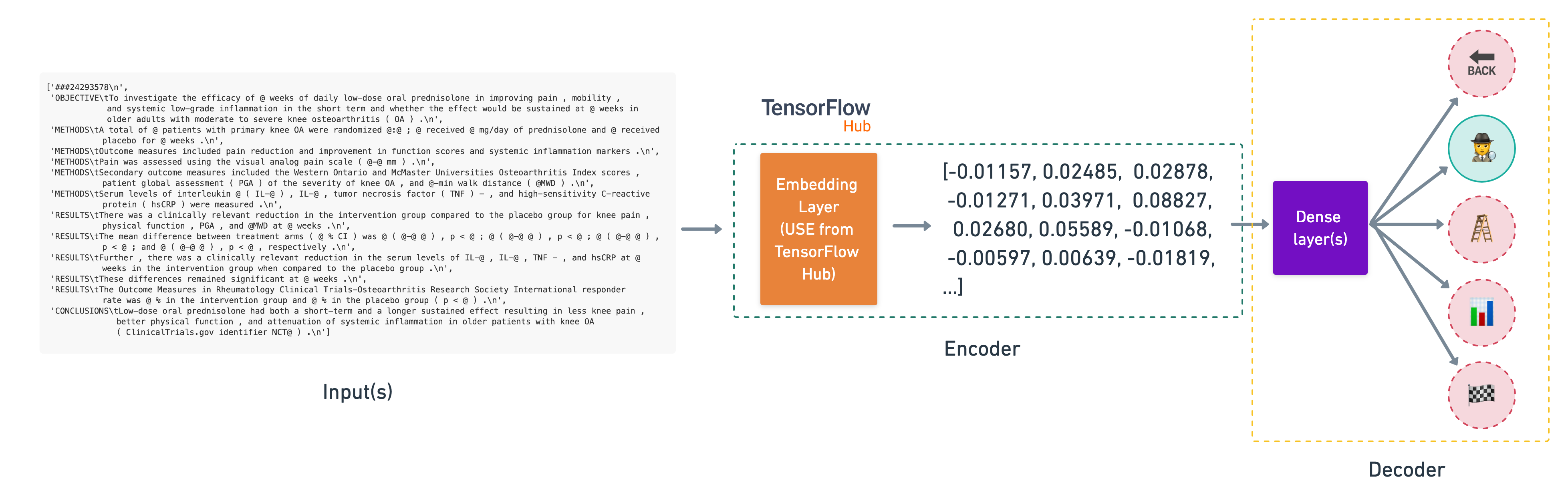 The feature extractor model we're building using a pretrained embedding from TensorFlow Hub.
To download the pretrained USE into a layer we can use in our model, we can use the hub.KerasLayer class.
We'll keep the pretrained embeddings frozen (by setting trainable=False) and add a trainable couple of layers on the top to tailor the model outputs to our own data.
🔑 Note: Due to having to download a relatively large model (~916MB), the cell below may take a little while to run.
# Download pretrained TensorFlow Hub USE
import tensorflow_hub as hub
tf_hub_embedding_layer = hub.KerasLayer("https://tfhub.dev/google/universal-sentence-encoder/4",
                                        trainable=False,
                                        name="universal_sentence_encoder")
Beautiful, now our pretrained USE is downloaded and instantiated as a hub.KerasLayer instance, let's test it out on a random sentence.
# Test out the embedding on a random sentence
random_training_sentence = random.choice(train_sentences)
print(f"Random training sentence:\n{random_training_sentence}\n")
use_embedded_sentence = tf_hub_embedding_layer([random_training_sentence])
print(f"Sentence after embedding:\n{use_embedded_sentence[0][:30]} (truncated output)...\n")
print(f"Length of sentence embedding:\n{len(use_embedded_sentence[0])}")
Random training sentence:
our data justify the need for personalized integrated antioxidant and energy correction therapy .

Sentence after embedding:
[-0.03416213 -0.05093268 -0.07358423  0.04783727 -0.05375864  0.07531483
 -0.0618328  -0.00023192  0.05290754  0.00731164  0.02909756 -0.03293613
 -0.05592315  0.02519475 -0.08728898 -0.02306924 -0.06509812  0.01185254
 -0.05143833 -0.01459878  0.03741732  0.05964429  0.03533797  0.05038223
  0.00830391 -0.05242855  0.05673083 -0.06287023  0.08674113  0.06334175] (truncated output)...

Length of sentence embedding:
512
Nice! As we mentioned before the pretrained USE module from TensorFlow Hub takes care of tokenizing our text for us and outputs a 512 dimensional embedding vector.
Let's put together and compile a model using our tf_hub_embedding_layer.
Building and fitting an NLP feature extraction model from TensorFlow Hub
# Define feature extractor model using TF Hub layer
inputs = layers.Input(shape=[], dtype=tf.string)
pretrained_embedding = tf_hub_embedding_layer(inputs) # tokenize text and create embedding
x = layers.Dense(128, activation="relu")(pretrained_embedding) # add a fully connected layer on top of the embedding
# Note: you could add more layers here if you wanted to
outputs = layers.Dense(5, activation="softmax")(x) # create the output layer
model_2 = tf.keras.Model(inputs=inputs,
                        outputs=outputs)

# Compile the model
model_2.compile(loss="categorical_crossentropy",
                optimizer=tf.keras.optimizers.Adam(),
                metrics=["accuracy"])
# Get a summary of the model
model_2.summary()
Model: "model_1"
_________________________________________________________________
 Layer (type)                Output Shape              Param #
=================================================================
 input_2 (InputLayer)        [(None,)]                 0

 universal_sentence_encoder   (None, 512)              256797824
 (KerasLayer)

 dense_1 (Dense)             (None, 128)               65664

 dense_2 (Dense)             (None, 5)                 645

=================================================================
Total params: 256,864,133
Trainable params: 66,309
Non-trainable params: 256,797,824
_________________________________________________________________
Checking the summary of our model we can see there's a large number of total parameters, however, the majority of these are non-trainable. This is because we set training=False when we instatiated our USE feature extractor layer.
So when we train our model, only the top two output layers will be trained.
# Fit feature extractor model for 3 epochs
model_2.fit(train_dataset,
            steps_per_epoch=int(0.1 * len(train_dataset)),
            epochs=3,
            validation_data=valid_dataset,
            validation_steps=int(0.1 * len(valid_dataset)))
Epoch 1/3
562/562 [==============================] - 9s 11ms/step - loss: 0.9207 - accuracy: 0.6496 - val_loss: 0.7936 - val_accuracy: 0.6908
Epoch 2/3
562/562 [==============================] - 6s 10ms/step - loss: 0.7659 - accuracy: 0.7047 - val_loss: 0.7499 - val_accuracy: 0.7074
Epoch 3/3
562/562 [==============================] - 6s 11ms/step - loss: 0.7471 - accuracy: 0.7145 - val_loss: 0.7328 - val_accuracy: 0.7178
<keras.callbacks.History at 0x7efb005bdff0>
# Evaluate on whole validation dataset
model_2.evaluate(valid_dataset)
945/945 [==============================] - 8s 8ms/step - loss: 0.7349 - accuracy: 0.7161
[0.7349329590797424, 0.7161061763763428]
Since we aren't training our own custom embedding layer, training is much quicker.
Let's make some predictions and evaluate our feature extraction model.
# Make predictions with feature extraction model
model_2_pred_probs = model_2.predict(valid_dataset)
model_2_pred_probs
945/945 [==============================] - 8s 8ms/step
array([[4.1435534e-01, 3.6443055e-01, 2.5627650e-03, 2.1054386e-01,
        8.1075458e-03],
       [3.4644338e-01, 4.7939345e-01, 4.0907143e-03, 1.6641928e-01,
        3.6531438e-03],
       [2.3935708e-01, 1.6314813e-01, 1.9130943e-02, 5.4523116e-01,
        3.3132695e-02],
       ...,
       [2.2427505e-03, 5.5871238e-03, 4.6554163e-02, 7.6473231e-04,
        9.4485116e-01],
       [3.8972907e-03, 4.4690356e-02, 2.0484674e-01, 1.4869794e-03,
        7.4507862e-01],
       [1.5384717e-01, 2.5815260e-01, 5.2709770e-01, 7.3189661e-03,
        5.3583570e-02]], dtype=float32)
# Convert the predictions with feature extraction model to classes
model_2_preds = tf.argmax(model_2_pred_probs, axis=1)
model_2_preds
<tf.Tensor: shape=(30212,), dtype=int64, numpy=array([0, 1, 3, ..., 4, 4, 2])>
# Calculate results from TF Hub pretrained embeddings results on validation set
model_2_results = calculate_results(y_true=val_labels_encoded,
                                    y_pred=model_2_preds)
model_2_results
{'accuracy': 71.61061829736528,
 'precision': 0.7161610082576743,
 'recall': 0.7161061829736528,
 'f1': 0.7128311588798425}
Model 3: Conv1D with character embeddings
Creating a character-level tokenizer
The Neural Networks for Joint Sentence Classification in Medical Paper Abstracts paper mentions their model uses a hybrid of token and character embeddings.
We've built models with a custom token embedding and a pretrained token embedding, how about we build one using a character embedding?
The difference between a character and token embedding is that the character embedding is created using sequences split into characters (e.g. hello -> [h, e, l, l, o]) where as a token embedding is created on sequences split into tokens.
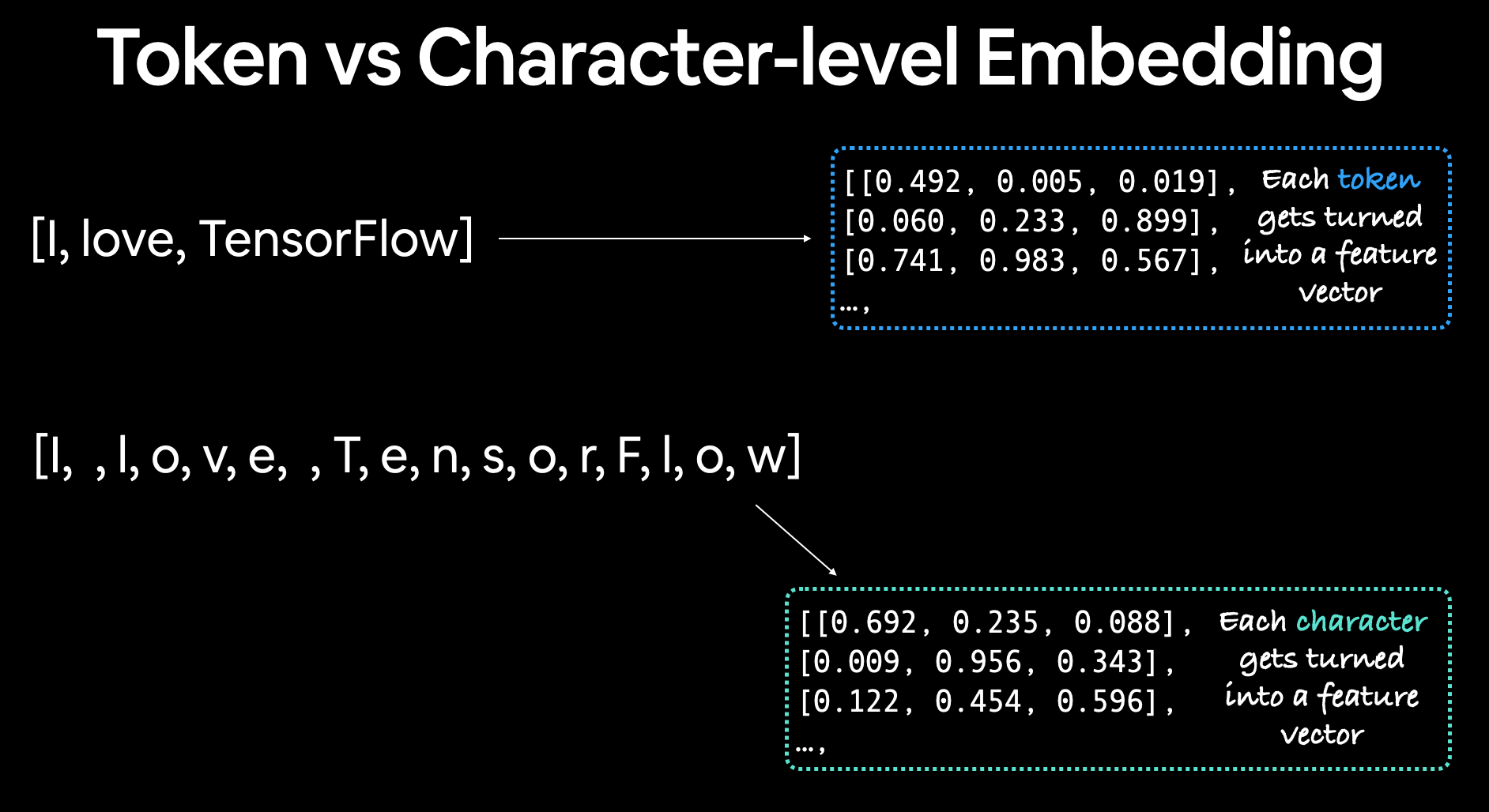 Token level embeddings split sequences into tokens (words) and embeddings each of them, character embeddings split sequences into characters and creates a feature vector for each.
We can create a character-level embedding by first vectorizing our sequences (after they've been split into characters) using the TextVectorization class and then passing those vectorized sequences through an Embedding layer.
Before we can vectorize our sequences on a character-level we'll need to split them into characters. Let's write a function to do so.
# Make function to split sentences into characters
def split_chars(text):
  return " ".join(list(text))

# Test splitting non-character-level sequence into characters
split_chars(random_training_sentence)
'o u r d a t a j u s t i f y t h e n e e d f o r p e r s o n a l i z e d i n t e g r a t e d a n t i o x i d a n t a n d e n e r g y c o r r e c t i o n t h e r a p y .'
Great! Looks like our character-splitting function works. Let's create character-level datasets by splitting our sequence datasets into characters.
# Split sequence-level data splits into character-level data splits
train_chars = [split_chars(sentence) for sentence in train_sentences]
val_chars = [split_chars(sentence) for sentence in val_sentences]
test_chars = [split_chars(sentence) for sentence in test_sentences]
print(train_chars[0])
t o i n v e s t i g a t e t h e e f f i c a c y o f @ w e e k s o f d a i l y l o w - d o s e o r a l p r e d n i s o l o n e i n i m p r o v i n g p a i n , m o b i l i t y , a n d s y s t e m i c l o w - g r a d e i n f l a m m a t i o n i n t h e s h o r t t e r m a n d w h e t h e r t h e e f f e c t w o u l d b e s u s t a i n e d a t @ w e e k s i n o l d e r a d u l t s w i t h m o d e r a t e t o s e v e r e k n e e o s t e o a r t h r i t i s ( o a ) .
To figure out how long our vectorized character sequences should be, let's check the distribution of our character sequence lengths.
# What's the average character length?
char_lens = [len(sentence) for sentence in train_sentences]
mean_char_len = np.mean(char_lens)
mean_char_len
149.3662574983337
# Check the distribution of our sequences at character-level
import matplotlib.pyplot as plt
plt.hist(char_lens, bins=7);

Okay, looks like most of our sequences are between 0 and 200 characters long.
Let's use NumPy's percentile to figure out what length covers 95% of our sequences.
# Find what character length covers 95% of sequences
output_seq_char_len = int(np.percentile(char_lens, 95))
output_seq_char_len
290
Wonderful, now we know the sequence length which covers 95% of sequences, we'll use that in our TextVectorization layer as the output_sequence_length parameter.
🔑 Note: You can experiment here to figure out what the optimal
output_sequence_lengthshould be, perhaps using the mean results in as good results as using the 95% percentile.
We'll set max_tokens (the total number of different characters in our sequences) to 28, in other words, 26 letters of the alphabet + space + OOV (out of vocabulary or unknown) tokens.
# Get all keyboard characters for char-level embedding
import string
alphabet = string.ascii_lowercase + string.digits + string.punctuation
alphabet
'abcdefghijklmnopqrstuvwxyz0123456789!"#$%&\'()*+,-./:;<=>?@[\\]^_`{|}~'
# Create char-level token vectorizer instance
NUM_CHAR_TOKENS = len(alphabet) + 2 # num characters in alphabet + space + OOV token
char_vectorizer = TextVectorization(max_tokens=NUM_CHAR_TOKENS,
                                    output_sequence_length=output_seq_char_len,
                                    standardize="lower_and_strip_punctuation",
                                    name="char_vectorizer")

# Adapt character vectorizer to training characters
char_vectorizer.adapt(train_chars)
Nice! Now we've adapted our char_vectorizer to our character-level sequences, let's check out some characteristics about it using the get_vocabulary() method.
# Check character vocabulary characteristics
char_vocab = char_vectorizer.get_vocabulary()
print(f"Number of different characters in character vocab: {len(char_vocab)}")
print(f"5 most common characters: {char_vocab[:5]}")
print(f"5 least common characters: {char_vocab[-5:]}")
Number of different characters in character vocab: 28
5 most common characters: ['', '[UNK]', 'e', 't', 'i']
5 least common characters: ['k', 'x', 'z', 'q', 'j']
We can also test it on random sequences of characters to make sure it's working.
# Test out character vectorizer
random_train_chars = random.choice(train_chars)
print(f"Charified text:\n{random_train_chars}")
print(f"\nLength of chars: {len(random_train_chars.split())}")
vectorized_chars = char_vectorizer([random_train_chars])
print(f"\nVectorized chars:\n{vectorized_chars}")
print(f"\nLength of vectorized chars: {len(vectorized_chars[0])}")
Charified text:
e x a m i n e   t h e   r e l a t i o n s h i p   o f   d e m o g r a p h i c s   a n d   h e a l t h   c o n d i t i o n s   ,   a l o n e   a n d   i n   c o m b i n a t i o n   ,   o n   o b j e c t i v e   m e a s u r e s   o f   c o g n i t i v e   f u n c t i o n   i n   a   l a r g e   s a m p l e   o f   c o m m u n i t y - d w e l l i n g   o l d e r   a d u l t s   .

Length of chars: 162

Vectorized chars:
[[ 2 24  5 15  4  6  2  3 13  2  8  2 12  5  3  4  7  6  9 13  4 14  7 17
  10  2 15  7 18  8  5 14 13  4 11  9  5  6 10 13  2  5 12  3 13 11  7  6
  10  4  3  4  7  6  9  5 12  7  6  2  5  6 10  4  6 11  7 15 22  4  6  5
   3  4  7  6  7  6  7 22 27  2 11  3  4 21  2 15  2  5  9 16  8  2  9  7
  17 11  7 18  6  4  3  4 21  2 17 16  6 11  3  4  7  6  4  6  5 12  5  8
  18  2  9  5 15 14 12  2  7 17 11  7 15 15 16  6  4  3 19 10 20  2 12 12
   4  6 18  7 12 10  2  8  5 10 16 12  3  9  0  0  0  0  0  0  0  0  0  0
   0  0  0  0  0  0  0  0  0  0  0  0  0  0  0  0  0  0  0  0  0  0  0  0
   0  0  0  0  0  0  0  0  0  0  0  0  0  0  0  0  0  0  0  0  0  0  0  0
   0  0  0  0  0  0  0  0  0  0  0  0  0  0  0  0  0  0  0  0  0  0  0  0
   0  0  0  0  0  0  0  0  0  0  0  0  0  0  0  0  0  0  0  0  0  0  0  0
   0  0  0  0  0  0  0  0  0  0  0  0  0  0  0  0  0  0  0  0  0  0  0  0
   0  0]]

Length of vectorized chars: 290
You'll notice sequences with a length shorter than 290 (output_seq_char_length) get padded with zeros on the end, this ensures all sequences passed to our model are the same length.
Also, due to the standardize parameter of TextVectorization being "lower_and_strip_punctuation" and the split parameter being "whitespace" by default, symbols (such as @) and spaces are removed.
🔑 Note: If you didn't want punctuation to be removed (keep the
@,%etc), you can create a custom standardization callable and pass it as thestandardizeparameter. See theTextVectorizationlayer documentation for more.
Creating a character-level embedding
We've got a way to vectorize our character-level sequences, now's time to create a character-level embedding.
Just like our custom token embedding, we can do so using the tensorflow.keras.layers.Embedding class.
Our character-level embedding layer requires an input dimension and output dimension.
The input dimension (input_dim) will be equal to the number of different characters in our char_vocab (28). And since we're following the structure of the model in Figure 1 of Neural Networks for Joint Sentence Classification
in Medical Paper Abstracts, the output dimension of the character embedding (output_dim) will be 25.
# Create char embedding layer
char_embed = layers.Embedding(input_dim=NUM_CHAR_TOKENS, # number of different characters
                              output_dim=25, # embedding dimension of each character (same as Figure 1 in https://arxiv.org/pdf/1612.05251.pdf)
                              mask_zero=False, # don't use masks (this messes up model_5 if set to True)
                              name="char_embed")

# Test out character embedding layer
print(f"Charified text (before vectorization and embedding):\n{random_train_chars}\n")
char_embed_example = char_embed(char_vectorizer([random_train_chars]))
print(f"Embedded chars (after vectorization and embedding):\n{char_embed_example}\n")
print(f"Character embedding shape: {char_embed_example.shape}")
Charified text (before vectorization and embedding):
e x a m i n e   t h e   r e l a t i o n s h i p   o f   d e m o g r a p h i c s   a n d   h e a l t h   c o n d i t i o n s   ,   a l o n e   a n d   i n   c o m b i n a t i o n   ,   o n   o b j e c t i v e   m e a s u r e s   o f   c o g n i t i v e   f u n c t i o n   i n   a   l a r g e   s a m p l e   o f   c o m m u n i t y - d w e l l i n g   o l d e r   a d u l t s   .

Embedded chars (after vectorization and embedding):
[[[-0.0242999  -0.04380112  0.03424067 ... -0.00923825 -0.03137535
    0.04647223]
  [ 0.03587342 -0.03863243 -0.03250255 ... -0.01955168  0.03022561
   -0.01134545]
  [ 0.04515156  0.0074586   0.04069341 ... -0.01211466 -0.02348533
    0.03110148]
  ...
  [-0.04492947  0.00582002  0.02089256 ...  0.02795838 -0.00649694
   -0.03568561]
  [-0.04492947  0.00582002  0.02089256 ...  0.02795838 -0.00649694
   -0.03568561]
  [-0.04492947  0.00582002  0.02089256 ...  0.02795838 -0.00649694
   -0.03568561]]]

Character embedding shape: (1, 290, 25)
Wonderful! Each of the characters in our sequences gets turned into a 25 dimension embedding.
Building a Conv1D model to fit on character embeddings
Now we've got a way to turn our character-level sequences into numbers (char_vectorizer) as well as numerically represent them as an embedding (char_embed) let's test how effective they are at encoding the information in our sequences by creating a character-level sequence model.
The model will have the same structure as our custom token embedding model (model_1) except it'll take character-level sequences as input instead of token-level sequences.
Input (character-level text) -> Tokenize -> Embedding -> Layers (Conv1D, GlobalMaxPool1D) -> Output (label probability)
# Make Conv1D on chars only
inputs = layers.Input(shape=(1,), dtype="string")
char_vectors = char_vectorizer(inputs)
char_embeddings = char_embed(char_vectors)
x = layers.Conv1D(64, kernel_size=5, padding="same", activation="relu")(char_embeddings)
x = layers.GlobalMaxPool1D()(x)
outputs = layers.Dense(num_classes, activation="softmax")(x)
model_3 = tf.keras.Model(inputs=inputs,
                         outputs=outputs,
                         name="model_3_conv1D_char_embedding")

# Compile model
model_3.compile(loss="categorical_crossentropy",
                optimizer=tf.keras.optimizers.Adam(),
                metrics=["accuracy"])
# Check the summary of conv1d_char_model
model_3.summary()
Model: "model_3_conv1D_char_embedding"
_________________________________________________________________
 Layer (type)                Output Shape              Param #
=================================================================
 input_3 (InputLayer)        [(None, 1)]               0

 char_vectorizer (TextVector  (None, 290)              0
 ization)

 char_embed (Embedding)      (None, 290, 25)           1750

 conv1d_1 (Conv1D)           (None, 290, 64)           8064

 global_max_pooling1d (Globa  (None, 64)               0
 lMaxPooling1D)

 dense_3 (Dense)             (None, 5)                 325

=================================================================
Total params: 10,139
Trainable params: 10,139
Non-trainable params: 0
_________________________________________________________________
Before fitting our model on the data, we'll create char-level batched PrefetchedDataset's.
# Create char datasets
train_char_dataset = tf.data.Dataset.from_tensor_slices((train_chars, train_labels_one_hot)).batch(32).prefetch(tf.data.AUTOTUNE)
val_char_dataset = tf.data.Dataset.from_tensor_slices((val_chars, val_labels_one_hot)).batch(32).prefetch(tf.data.AUTOTUNE)

train_char_dataset
<_PrefetchDataset element_spec=(TensorSpec(shape=(None,), dtype=tf.string, name=None), TensorSpec(shape=(None, 5), dtype=tf.float64, name=None))>
Just like our token-level sequence model, to save time with our experiments, we'll fit the character-level model on 10% of batches.
# Fit the model on chars only
model_3_history = model_3.fit(train_char_dataset,
                              steps_per_epoch=int(0.1 * len(train_char_dataset)),
                              epochs=3,
                              validation_data=val_char_dataset,
                              validation_steps=int(0.1 * len(val_char_dataset)))
Epoch 1/3
562/562 [==============================] - 5s 6ms/step - loss: 1.2876 - accuracy: 0.4835 - val_loss: 1.0503 - val_accuracy: 0.5934
Epoch 2/3
562/562 [==============================] - 3s 5ms/step - loss: 0.9992 - accuracy: 0.6053 - val_loss: 0.9375 - val_accuracy: 0.6330
Epoch 3/3
562/562 [==============================] - 2s 4ms/step - loss: 0.9217 - accuracy: 0.6366 - val_loss: 0.8723 - val_accuracy: 0.6576
# Evaluate model_3 on whole validation char dataset
model_3.evaluate(val_char_dataset)
945/945 [==============================] - 3s 3ms/step - loss: 0.8830 - accuracy: 0.6543
[0.8829597234725952, 0.6543095707893372]
Nice! Looks like our character-level model is working, let's make some predictions with it and evaluate them.
# Make predictions with character model only
model_3_pred_probs = model_3.predict(val_char_dataset)
model_3_pred_probs
945/945 [==============================] - 2s 2ms/step
array([[0.16555832, 0.40962285, 0.10694715, 0.24029495, 0.07757679],
       [0.15813953, 0.53640217, 0.01517234, 0.26619416, 0.02409185],
       [0.12398545, 0.23686218, 0.16067787, 0.41156322, 0.06691124],
       ...,
       [0.03653853, 0.05342488, 0.29759905, 0.0883414 , 0.52409613],
       [0.07498587, 0.1934537 , 0.29657316, 0.10817684, 0.3268104 ],
       [0.3868036 , 0.46745342, 0.07763865, 0.04975864, 0.01834559]],
      dtype=float32)
# Convert predictions to classes
model_3_preds = tf.argmax(model_3_pred_probs, axis=1)
model_3_preds
<tf.Tensor: shape=(30212,), dtype=int64, numpy=array([1, 1, 3, ..., 4, 4, 1])>
# Calculate Conv1D char only model results
model_3_results = calculate_results(y_true=val_labels_encoded,
                                        y_pred=model_3_preds)
model_3_results
{'accuracy': 65.4309545875811,
 'precision': 0.6475618110732863,
 'recall': 0.6543095458758109,
 'f1': 0.6428526324260226}
Model 4: Combining pretrained token embeddings + character embeddings (hybrid embedding layer)
Alright, now things are going to get spicy.
In moving closer to build a model similar to the one in Figure 1 of Neural Networks for Joint Sentence Classification in Medical Paper Abstracts, it's time we tackled the hybrid token embedding layer they speak of.
This hybrid token embedding layer is a combination of token embeddings and character embeddings. In other words, they create a stacked embedding to represent sequences before passing them to the sequence label prediction layer.
So far we've built two models which have used token and character-level embeddings, however, these two models have used each of these embeddings exclusively.
To start replicating (or getting close to replicating) the model in Figure 1, we're going to go through the following steps:
- Create a token-level model (similar to
model_1) - Create a character-level model (similar to
model_3with a slight modification to reflect the paper) - Combine (using
layers.Concatenate) the outputs of 1 and 2 - Build a series of output layers on top of 3 similar to Figure 1 and section 4.2 of Neural Networks for Joint Sentence Classification in Medical Paper Abstracts
- Construct a model which takes token and character-level sequences as input and produces sequence label probabilities as output
# 1. Setup token inputs/model
token_inputs = layers.Input(shape=[], dtype=tf.string, name="token_input")
token_embeddings = tf_hub_embedding_layer(token_inputs)
token_output = layers.Dense(128, activation="relu")(token_embeddings)
token_model = tf.keras.Model(inputs=token_inputs,
                             outputs=token_output)

# 2. Setup char inputs/model
char_inputs = layers.Input(shape=(1,), dtype=tf.string, name="char_input")
char_vectors = char_vectorizer(char_inputs)
char_embeddings = char_embed(char_vectors)
char_bi_lstm = layers.Bidirectional(layers.LSTM(25))(char_embeddings) # bi-LSTM shown in Figure 1 of https://arxiv.org/pdf/1612.05251.pdf
char_model = tf.keras.Model(inputs=char_inputs,
                            outputs=char_bi_lstm)

# 3. Concatenate token and char inputs (create hybrid token embedding)
token_char_concat = layers.Concatenate(name="token_char_hybrid")([token_model.output,
                                                                  char_model.output])

# 4. Create output layers - addition of dropout discussed in 4.2 of https://arxiv.org/pdf/1612.05251.pdf
combined_dropout = layers.Dropout(0.5)(token_char_concat)
combined_dense = layers.Dense(200, activation="relu")(combined_dropout) # slightly different to Figure 1 due to different shapes of token/char embedding layers
final_dropout = layers.Dropout(0.5)(combined_dense)
output_layer = layers.Dense(num_classes, activation="softmax")(final_dropout)

# 5. Construct model with char and token inputs
model_4 = tf.keras.Model(inputs=[token_model.input, char_model.input],
                         outputs=output_layer,
                         name="model_4_token_and_char_embeddings")
Woah... There's a lot going on here, let's get a summary and plot our model to visualize what's happening.
# Get summary of token and character model
model_4.summary()
Model: "model_4_token_and_char_embeddings"
__________________________________________________________________________________________________
 Layer (type)                   Output Shape         Param #     Connected to
==================================================================================================
 char_input (InputLayer)        [(None, 1)]          0           []

 token_input (InputLayer)       [(None,)]            0           []

 char_vectorizer (TextVectoriza  (None, 290)         0           ['char_input[0][0]']
 tion)

 universal_sentence_encoder (Ke  (None, 512)         256797824   ['token_input[0][0]']
 rasLayer)

 char_embed (Embedding)         (None, 290, 25)      1750        ['char_vectorizer[1][0]']

 dense_4 (Dense)                (None, 128)          65664       ['universal_sentence_encoder[1][0
                                                                 ]']

 bidirectional (Bidirectional)  (None, 50)           10200       ['char_embed[1][0]']

 token_char_hybrid (Concatenate  (None, 178)         0           ['dense_4[0][0]',
 )                                                                'bidirectional[0][0]']

 dropout (Dropout)              (None, 178)          0           ['token_char_hybrid[0][0]']

 dense_5 (Dense)                (None, 200)          35800       ['dropout[0][0]']

 dropout_1 (Dropout)            (None, 200)          0           ['dense_5[0][0]']

 dense_6 (Dense)                (None, 5)            1005        ['dropout_1[0][0]']

==================================================================================================
Total params: 256,912,243
Trainable params: 114,419
Non-trainable params: 256,797,824
__________________________________________________________________________________________________
# Plot hybrid token and character model
from tensorflow.keras.utils import plot_model
plot_model(model_4)

Now that's a good looking model. Let's compile it just as we have the rest of our models.
🔑 Note: Section 4.2 of Neural Networks for Joint Sentence Classification in Medical Paper Abstracts mentions using the SGD (stochastic gradient descent) optimizer, however, to stay consistent with our other models, we're going to use the Adam optimizer. As an exercise, you could try using
tf.keras.optimizers.SGDinstead oftf.keras.optimizers.Adamand compare the results.
# Compile token char model
model_4.compile(loss="categorical_crossentropy",
                optimizer=tf.keras.optimizers.Adam(), # section 4.2 of https://arxiv.org/pdf/1612.05251.pdf mentions using SGD but we'll stick with Adam
                metrics=["accuracy"])
And again, to keep our experiments fast, we'll fit our token-character-hybrid model on 10% of training and validate on 10% of validation batches. However, the difference with this model is that it requires two inputs, token-level sequences and character-level sequences.
We can do this by create a tf.data.Dataset with a tuple as it's first input, for example:
((token_data, char_data), (label))
Let's see it in action.
Combining token and character data into a tf.data dataset
# Combine chars and tokens into a dataset
train_char_token_data = tf.data.Dataset.from_tensor_slices((train_sentences, train_chars)) # make data
train_char_token_labels = tf.data.Dataset.from_tensor_slices(train_labels_one_hot) # make labels
train_char_token_dataset = tf.data.Dataset.zip((train_char_token_data, train_char_token_labels)) # combine data and labels

# Prefetch and batch train data
train_char_token_dataset = train_char_token_dataset.batch(32).prefetch(tf.data.AUTOTUNE)

# Repeat same steps validation data
val_char_token_data = tf.data.Dataset.from_tensor_slices((val_sentences, val_chars))
val_char_token_labels = tf.data.Dataset.from_tensor_slices(val_labels_one_hot)
val_char_token_dataset = tf.data.Dataset.zip((val_char_token_data, val_char_token_labels))
val_char_token_dataset = val_char_token_dataset.batch(32).prefetch(tf.data.AUTOTUNE)
# Check out training char and token embedding dataset
train_char_token_dataset, val_char_token_dataset
(<_PrefetchDataset element_spec=((TensorSpec(shape=(None,), dtype=tf.string, name=None), TensorSpec(shape=(None,), dtype=tf.string, name=None)), TensorSpec(shape=(None, 5), dtype=tf.float64, name=None))>,
 <_PrefetchDataset element_spec=((TensorSpec(shape=(None,), dtype=tf.string, name=None), TensorSpec(shape=(None,), dtype=tf.string, name=None)), TensorSpec(shape=(None, 5), dtype=tf.float64, name=None))>)
Fitting a model on token and character-level sequences
# Fit the model on tokens and chars
model_4_history = model_4.fit(train_char_token_dataset, # train on dataset of token and characters
                              steps_per_epoch=int(0.1 * len(train_char_token_dataset)),
                              epochs=3,
                              validation_data=val_char_token_dataset,
                              validation_steps=int(0.1 * len(val_char_token_dataset)))
Epoch 1/3
562/562 [==============================] - 22s 28ms/step - loss: 0.9718 - accuracy: 0.6148 - val_loss: 0.7762 - val_accuracy: 0.7015
Epoch 2/3
562/562 [==============================] - 14s 25ms/step - loss: 0.7930 - accuracy: 0.6936 - val_loss: 0.7155 - val_accuracy: 0.7301
Epoch 3/3
562/562 [==============================] - 14s 25ms/step - loss: 0.7680 - accuracy: 0.7040 - val_loss: 0.6885 - val_accuracy: 0.7374
# Evaluate on the whole validation dataset
model_4.evaluate(val_char_token_dataset)
945/945 [==============================] - 13s 13ms/step - loss: 0.6905 - accuracy: 0.7350
[0.6904993653297424, 0.7350390553474426]
Nice! Our token-character hybrid model has come to life!
To make predictions with it, since it takes multiplie inputs, we can pass the predict() method a tuple of token-level sequences and character-level sequences.
We can then evaluate the predictions as we've done before.
# Make predictions using the token-character model hybrid
model_4_pred_probs = model_4.predict(val_char_token_dataset)
model_4_pred_probs
945/945 [==============================] - 13s 13ms/step
array([[3.50879818e-01, 4.52533990e-01, 1.95086596e-03, 1.89795882e-01,
        4.83940262e-03],
       [2.65543371e-01, 5.95941365e-01, 3.22520477e-03, 1.32380798e-01,
        2.90922332e-03],
       [2.61086196e-01, 1.19279526e-01, 5.44379167e-02, 5.30372798e-01,
        3.48235779e-02],
       ...,
       [3.58209974e-04, 5.53221209e-03, 6.14999533e-02, 1.56954877e-04,
        9.32452679e-01],
       [5.82700176e-03, 6.14563487e-02, 2.22319663e-01, 2.89280107e-03,
        7.07504213e-01],
       [2.78134555e-01, 2.37935275e-01, 3.98698568e-01, 2.44974717e-02,
        6.07340895e-02]], dtype=float32)
# Turn prediction probabilities into prediction classes
model_4_preds = tf.argmax(model_4_pred_probs, axis=1)
model_4_preds
<tf.Tensor: shape=(30212,), dtype=int64, numpy=array([1, 1, 3, ..., 4, 4, 2])>
# Get results of token-char-hybrid model
model_4_results = calculate_results(y_true=val_labels_encoded,
                                    y_pred=model_4_preds)
model_4_results
{'accuracy': 73.5039057328214,
 'precision': 0.737718289862149,
 'recall': 0.735039057328214,
 'f1': 0.7310235703293549}
Model 5: Transfer Learning with pretrained token embeddings + character embeddings + positional embeddings
It seems like combining token embeddings and character embeddings gave our model a little performance boost.
But there's one more piece of the puzzle we can add in.
What if we engineered our own features into the model?
Meaning, what if we took our own knowledge about the data and encoded it in a numerical way to give our model more information about our samples?
The process of applying your own knowledge to build features as input to a model is called feature engineering.
Can you think of something important about the sequences we're trying to classify?
If you were to look at an abstract, would you expect the sentences to appear in order? Or does it make sense if they were to appear sequentially? For example, sequences labelled CONCLUSIONS at the beggining and sequences labelled OBJECTIVE at the end?
Abstracts typically come in a sequential order, such as:
OBJECTIVE...METHODS...METHODS...METHODS...RESULTS...CONCLUSIONS...
Or
BACKGROUND...OBJECTIVE...METHODS...METHODS...RESULTS...RESULTS...CONCLUSIONS...CONCLUSIONS...
Of course, we can't engineer the sequence labels themselves into the training data (we don't have these at test time), but we can encode the order of a set of sequences in an abstract.
For example,
Sentence 1 of 10...Sentence 2 of 10...Sentence 3 of 10...Sentence 4 of 10...- ...
You might've noticed this when we created our preprocess_text_with_line_numbers() function. When we read in a text file of abstracts, we counted the number of lines in an abstract as well as the number of each line itself.
Doing this led to the "line_number" and "total_lines" columns of our DataFrames.
# Inspect training dataframe
train_df.head()
| target | text | line_number | total_lines | |
|---|---|---|---|---|
| 0 | OBJECTIVE | to investigate the efficacy of @ weeks of dail... | 0 | 11 |
| 1 | METHODS | a total of @ patients with primary knee oa wer... | 1 | 11 |
| 2 | METHODS | outcome measures included pain reduction and i... | 2 | 11 |
| 3 | METHODS | pain was assessed using the visual analog pain... | 3 | 11 |
| 4 | METHODS | secondary outcome measures included the wester... | 4 | 11 |
The "line_number" and "total_lines" columns are features which didn't necessarily come with the training data but can be passed to our model as a positional embedding. In other words, the positional embedding is where the sentence appears in an abstract.
We can use these features because they will be available at test time.
 Since abstracts typically have a sequential order about them (for example, background, objective, methods, results, conclusion), it makes sense to add the line number of where a particular sentence occurs to our model. The beautiful thing is, these features will be available at test time (we can just count the number of sentences in an abstract and the number of each one).
Meaning, if we were to predict the labels of sequences in an abstract our model had never seen, we could count the number of lines and the track the position of each individual line and pass it to our model.
🛠 Exercise: Another way of creating our positional embedding feature would be to combine the
"line_number"and"total_lines"columns into one, for example a"line_position"column may contain values like1_of_11,2_of_11, etc. Where1_of_11would be the first line in an abstract 11 sentences long. After going through the following steps, you might want to revisit this positional embedding stage and see how a combined column of"line_position"goes against two separate columns.
Create positional embeddings
Okay, enough talk about positional embeddings, let's create them.
Since our "line_number" and "total_line" columns are already numerical, we could pass them as they are to our model.
But to avoid our model thinking a line with "line_number"=5 is five times greater than a line with "line_number"=1, we'll use one-hot-encoding to encode our "line_number" and "total_lines" features.
To do this, we can use the tf.one_hot utility.
tf.one_hot returns a one-hot-encoded tensor. It accepts an array (or tensor) as input and the depth parameter determines the dimension of the returned tensor.
To figure out what we should set the depth parameter to, let's investigate the distribution of the "line_number" column.
🔑 Note: When it comes to one-hot-encoding our features, Scikit-Learn's
OneHotEncoderclass is another viable option here.
# How many different line numbers are there?
train_df["line_number"].value_counts()
0     15000
1     15000
2     15000
3     15000
4     14992
5     14949
6     14758
7     14279
8     13346
9     11981
10    10041
11     7892
12     5853
13     4152
14     2835
15     1861
16     1188
17      751
18      462
19      286
20      162
21      101
22       66
23       33
24       22
25       14
26        7
27        4
28        3
29        1
30        1
Name: line_number, dtype: int64
# Check the distribution of "line_number" column
train_df.line_number.plot.hist()
<Axes: ylabel='Frequency'>

Looking at the distribution of the "line_number" column, it looks like the majority of lines have a position of 15 or less.
Knowing this, let's set the depth parameter of tf.one_hot to 15.
# Use TensorFlow to create one-hot-encoded tensors of our "line_number" column
train_line_numbers_one_hot = tf.one_hot(train_df["line_number"].to_numpy(), depth=15)
val_line_numbers_one_hot = tf.one_hot(val_df["line_number"].to_numpy(), depth=15)
test_line_numbers_one_hot = tf.one_hot(test_df["line_number"].to_numpy(), depth=15)
Setting the depth parameter of tf.one_hot to 15 means any sample with a "line_number" value of over 15 gets set to a tensor of all 0's, where as any sample with a "line_number" of under 15 gets turned into a tensor of all 0's but with a 1 at the index equal to the "line_number" value.
🔑 Note: We could create a one-hot tensor which has room for all of the potential values of
"line_number"(depth=30), however, this would end up in a tensor of double the size of our current one (depth=15) where the vast majority of values are 0. Plus, only ~2,000/180,000 samples have a"line_number"value of over 15. So we would not be gaining much information about our data for doubling our feature space. This kind of problem is called the curse of dimensionality. However, since this we're working with deep models, it might be worth trying to throw as much information at the model as possible and seeing what happens. I'll leave exploring values of thedepthparameter as an extension.
# Check one-hot encoded "line_number" feature samples
train_line_numbers_one_hot.shape, train_line_numbers_one_hot[:20]
(TensorShape([180040, 15]),
 <tf.Tensor: shape=(20, 15), dtype=float32, numpy=
 array([[1., 0., 0., 0., 0., 0., 0., 0., 0., 0., 0., 0., 0., 0., 0.],
        [0., 1., 0., 0., 0., 0., 0., 0., 0., 0., 0., 0., 0., 0., 0.],
        [0., 0., 1., 0., 0., 0., 0., 0., 0., 0., 0., 0., 0., 0., 0.],
        [0., 0., 0., 1., 0., 0., 0., 0., 0., 0., 0., 0., 0., 0., 0.],
        [0., 0., 0., 0., 1., 0., 0., 0., 0., 0., 0., 0., 0., 0., 0.],
        [0., 0., 0., 0., 0., 1., 0., 0., 0., 0., 0., 0., 0., 0., 0.],
        [0., 0., 0., 0., 0., 0., 1., 0., 0., 0., 0., 0., 0., 0., 0.],
        [0., 0., 0., 0., 0., 0., 0., 1., 0., 0., 0., 0., 0., 0., 0.],
        [0., 0., 0., 0., 0., 0., 0., 0., 1., 0., 0., 0., 0., 0., 0.],
        [0., 0., 0., 0., 0., 0., 0., 0., 0., 1., 0., 0., 0., 0., 0.],
        [0., 0., 0., 0., 0., 0., 0., 0., 0., 0., 1., 0., 0., 0., 0.],
        [0., 0., 0., 0., 0., 0., 0., 0., 0., 0., 0., 1., 0., 0., 0.],
        [1., 0., 0., 0., 0., 0., 0., 0., 0., 0., 0., 0., 0., 0., 0.],
        [0., 1., 0., 0., 0., 0., 0., 0., 0., 0., 0., 0., 0., 0., 0.],
        [0., 0., 1., 0., 0., 0., 0., 0., 0., 0., 0., 0., 0., 0., 0.],
        [0., 0., 0., 1., 0., 0., 0., 0., 0., 0., 0., 0., 0., 0., 0.],
        [0., 0., 0., 0., 1., 0., 0., 0., 0., 0., 0., 0., 0., 0., 0.],
        [0., 0., 0., 0., 0., 1., 0., 0., 0., 0., 0., 0., 0., 0., 0.],
        [0., 0., 0., 0., 0., 0., 1., 0., 0., 0., 0., 0., 0., 0., 0.],
        [0., 0., 0., 0., 0., 0., 0., 1., 0., 0., 0., 0., 0., 0., 0.]],
       dtype=float32)>)
We can do the same as we've done for our "line_number" column witht he "total_lines" column. First, let's find an appropriate value for the depth parameter of tf.one_hot.
# How many different numbers of lines are there?
train_df["total_lines"].value_counts()
11    24468
10    23639
12    22113
9     19400
13    18438
14    14610
8     12285
15    10768
7      7464
16     7429
17     5202
6      3353
18     3344
19     2480
20     1281
5      1146
21      770
22      759
23      264
4       215
24      200
25      182
26       81
28       58
3        32
30       31
27       28
Name: total_lines, dtype: int64
# Check the distribution of total lines
train_df.total_lines.plot.hist();
Looking at the distribution of our "total_lines" column, a value of 20 looks like it covers the majority of samples.
We can confirm this with np.percentile().
# Check the coverage of a "total_lines" value of 20
np.percentile(train_df.total_lines, 98) # a value of 20 covers 98% of samples
20.0
Beautiful! Plenty of converage. Let's one-hot-encode our "total_lines" column just as we did our "line_number" column.
# Use TensorFlow to create one-hot-encoded tensors of our "total_lines" column
train_total_lines_one_hot = tf.one_hot(train_df["total_lines"].to_numpy(), depth=20)
val_total_lines_one_hot = tf.one_hot(val_df["total_lines"].to_numpy(), depth=20)
test_total_lines_one_hot = tf.one_hot(test_df["total_lines"].to_numpy(), depth=20)

# Check shape and samples of total lines one-hot tensor
train_total_lines_one_hot.shape, train_total_lines_one_hot[:10]
(TensorShape([180040, 20]),
 <tf.Tensor: shape=(10, 20), dtype=float32, numpy=
 array([[0., 0., 0., 0., 0., 0., 0., 0., 0., 0., 0., 1., 0., 0., 0., 0.,
         0., 0., 0., 0.],
        [0., 0., 0., 0., 0., 0., 0., 0., 0., 0., 0., 1., 0., 0., 0., 0.,
         0., 0., 0., 0.],
        [0., 0., 0., 0., 0., 0., 0., 0., 0., 0., 0., 1., 0., 0., 0., 0.,
         0., 0., 0., 0.],
        [0., 0., 0., 0., 0., 0., 0., 0., 0., 0., 0., 1., 0., 0., 0., 0.,
         0., 0., 0., 0.],
        [0., 0., 0., 0., 0., 0., 0., 0., 0., 0., 0., 1., 0., 0., 0., 0.,
         0., 0., 0., 0.],
        [0., 0., 0., 0., 0., 0., 0., 0., 0., 0., 0., 1., 0., 0., 0., 0.,
         0., 0., 0., 0.],
        [0., 0., 0., 0., 0., 0., 0., 0., 0., 0., 0., 1., 0., 0., 0., 0.,
         0., 0., 0., 0.],
        [0., 0., 0., 0., 0., 0., 0., 0., 0., 0., 0., 1., 0., 0., 0., 0.,
         0., 0., 0., 0.],
        [0., 0., 0., 0., 0., 0., 0., 0., 0., 0., 0., 1., 0., 0., 0., 0.,
         0., 0., 0., 0.],
        [0., 0., 0., 0., 0., 0., 0., 0., 0., 0., 0., 1., 0., 0., 0., 0.,
         0., 0., 0., 0.]], dtype=float32)>)
Building a tribrid embedding model
Woohoo! Positional embedding tensors ready.
It's time to build the biggest model we've built yet. One which incorporates token embeddings, character embeddings and our newly crafted positional embeddings.
We'll be venturing into uncovered territory but there will be nothing here you haven't practiced before.
More specifically we're going to go through the following steps:
- Create a token-level model (similar to
model_1) - Create a character-level model (similar to
model_3with a slight modification to reflect the paper) - Create a
"line_number"model (takes in one-hot-encoded"line_number"tensor and passes it through a non-linear layer) - Create a
"total_lines"model (takes in one-hot-encoded"total_lines"tensor and passes it through a non-linear layer) - Combine (using
layers.Concatenate) the outputs of 1 and 2 into a token-character-hybrid embedding and pass it series of output to Figure 1 and section 4.2 of Neural Networks for Joint Sentence Classification in Medical Paper Abstracts - Combine (using
layers.Concatenate) the outputs of 3, 4 and 5 into a token-character-positional tribrid embedding - Create an output layer to accept the tribrid embedding and output predicted label probabilities
- Combine the inputs of 1, 2, 3, 4 and outputs of 7 into a
tf.keras.Model
Woah! That's alot... but nothing we're not capable of. Let's code it.
# 1. Token inputs
token_inputs = layers.Input(shape=[], dtype="string", name="token_inputs")
token_embeddings = tf_hub_embedding_layer(token_inputs)
token_outputs = layers.Dense(128, activation="relu")(token_embeddings)
token_model = tf.keras.Model(inputs=token_inputs,
                             outputs=token_outputs)

# 2. Char inputs
char_inputs = layers.Input(shape=(1,), dtype="string", name="char_inputs")
char_vectors = char_vectorizer(char_inputs)
char_embeddings = char_embed(char_vectors)
char_bi_lstm = layers.Bidirectional(layers.LSTM(32))(char_embeddings)
char_model = tf.keras.Model(inputs=char_inputs,
                            outputs=char_bi_lstm)

# 3. Line numbers inputs
line_number_inputs = layers.Input(shape=(15,), dtype=tf.int32, name="line_number_input")
x = layers.Dense(32, activation="relu")(line_number_inputs)
line_number_model = tf.keras.Model(inputs=line_number_inputs,
                                   outputs=x)

# 4. Total lines inputs
total_lines_inputs = layers.Input(shape=(20,), dtype=tf.int32, name="total_lines_input")
y = layers.Dense(32, activation="relu")(total_lines_inputs)
total_line_model = tf.keras.Model(inputs=total_lines_inputs,
                                  outputs=y)

# 5. Combine token and char embeddings into a hybrid embedding
combined_embeddings = layers.Concatenate(name="token_char_hybrid_embedding")([token_model.output,
                                                                              char_model.output])
z = layers.Dense(256, activation="relu")(combined_embeddings)
z = layers.Dropout(0.5)(z)

# 6. Combine positional embeddings with combined token and char embeddings into a tribrid embedding
z = layers.Concatenate(name="token_char_positional_embedding")([line_number_model.output,
                                                                total_line_model.output,
                                                                z])

# 7. Create output layer
output_layer = layers.Dense(5, activation="softmax", name="output_layer")(z)

# 8. Put together model
model_5 = tf.keras.Model(inputs=[line_number_model.input,
                                 total_line_model.input,
                                 token_model.input,
                                 char_model.input],
                         outputs=output_layer)
There's a lot going on here... let's visualize what's happening with a summary by plotting our model.
# Get a summary of our token, char and positional embedding model
model_5.summary()
Model: "model_8"
__________________________________________________________________________________________________
 Layer (type)                   Output Shape         Param #     Connected to
==================================================================================================
 char_inputs (InputLayer)       [(None, 1)]          0           []

 token_inputs (InputLayer)      [(None,)]            0           []

 char_vectorizer (TextVectoriza  (None, 290)         0           ['char_inputs[0][0]']
 tion)

 universal_sentence_encoder (Ke  (None, 512)         256797824   ['token_inputs[0][0]']
 rasLayer)

 char_embed (Embedding)         (None, 290, 25)      1750        ['char_vectorizer[2][0]']

 dense_7 (Dense)                (None, 128)          65664       ['universal_sentence_encoder[2][0
                                                                 ]']

 bidirectional_1 (Bidirectional  (None, 64)          14848       ['char_embed[2][0]']
 )

 token_char_hybrid_embedding (C  (None, 192)         0           ['dense_7[0][0]',
 oncatenate)                                                      'bidirectional_1[0][0]']

 line_number_input (InputLayer)  [(None, 15)]        0           []

 total_lines_input (InputLayer)  [(None, 20)]        0           []

 dense_10 (Dense)               (None, 256)          49408       ['token_char_hybrid_embedding[0][
                                                                 0]']

 dense_8 (Dense)                (None, 32)           512         ['line_number_input[0][0]']

 dense_9 (Dense)                (None, 32)           672         ['total_lines_input[0][0]']

 dropout_2 (Dropout)            (None, 256)          0           ['dense_10[0][0]']

 token_char_positional_embeddin  (None, 320)         0           ['dense_8[0][0]',
 g (Concatenate)                                                  'dense_9[0][0]',
                                                                  'dropout_2[0][0]']

 output_layer (Dense)           (None, 5)            1605        ['token_char_positional_embedding
                                                                 [0][0]']

==================================================================================================
Total params: 256,932,283
Trainable params: 134,459
Non-trainable params: 256,797,824
__________________________________________________________________________________________________
# Plot the token, char, positional embedding model
from tensorflow.keras.utils import plot_model
plot_model(model_5)

Visualizing the model makes it much easier to understand.
Essentially what we're doing is trying to encode as much information about our sequences as possible into various embeddings (the inputs to our model) so our model has the best chance to figure out what label belongs to a sequence (the outputs of our model).
You'll notice our model is looking very similar to the model shown in Figure 1 of Neural Networks for Joint Sentence Classification in Medical Paper Abstracts. However, a few differences still remain:
- We're using pretrained TensorFlow Hub token embeddings instead of GloVe emebddings.
- We're using a Dense layer on top of our token-character hybrid embeddings instead of a bi-LSTM layer.
- Section 3.1.3 of the paper mentions a label sequence optimization layer (which helps to make sure sequence labels come out in a respectable order) but it isn't shown in Figure 1. To makeup for the lack of this layer in our model, we've created the positional embeddings layers.
- Section 4.2 of the paper mentions the token and character embeddings are updated during training, our pretrained TensorFlow Hub embeddings remain frozen.
- The paper uses the
SGDoptimizer, we're going to stick withAdam.
All of the differences above are potential extensions of this project.
# Check which layers of our model are trainable or not
for layer in model_5.layers:
  print(layer, layer.trainable)
<keras.engine.input_layer.InputLayer object at 0x7efa4933cd60> True
<keras.engine.input_layer.InputLayer object at 0x7efa4933d120> True
<keras.layers.preprocessing.text_vectorization.TextVectorization object at 0x7efa49737cd0> True
<tensorflow_hub.keras_layer.KerasLayer object at 0x7efb801dc610> False
<keras.layers.core.embedding.Embedding object at 0x7efa4976d240> True
<keras.layers.core.dense.Dense object at 0x7efa4933d960> True
<keras.layers.rnn.bidirectional.Bidirectional object at 0x7efa493b9600> True
<keras.layers.merging.concatenate.Concatenate object at 0x7efa49222260> True
<keras.engine.input_layer.InputLayer object at 0x7efa493934f0> True
<keras.engine.input_layer.InputLayer object at 0x7efa493bac50> True
<keras.layers.core.dense.Dense object at 0x7efa49237190> True
<keras.layers.core.dense.Dense object at 0x7efa49737c70> True
<keras.layers.core.dense.Dense object at 0x7efa493d4130> True
<keras.layers.regularization.dropout.Dropout object at 0x7efa493bb220> True
<keras.layers.merging.concatenate.Concatenate object at 0x7efa492abfd0> True
<keras.layers.core.dense.Dense object at 0x7efa492c9420> True
Now our model is constructed, let's compile it.
This time, we're going to introduce a new parameter to our loss function called label_smoothing. Label smoothing helps to regularize our model (prevent overfitting) by making sure it doesn't get too focused on applying one particular label to a sample.
For example, instead of having an output prediction of:
[0.0, 0.0, 1.0, 0.0, 0.0]for a sample (the model is very confident the right label is index 2).
It's predictions will get smoothed to be something like:
[0.01, 0.01, 0.096, 0.01, 0.01]giving a small activation to each of the other labels, in turn, hopefully improving generalization.
📖 Resource: For more on label smoothing, see the great blog post by PyImageSearch, Label smoothing with Keras, TensorFlow, and Deep Learning.
# Compile token, char, positional embedding model
model_5.compile(loss=tf.keras.losses.CategoricalCrossentropy(label_smoothing=0.2), # add label smoothing (examples which are really confident get smoothed a little)
                optimizer=tf.keras.optimizers.Adam(),
                metrics=["accuracy"])
Create tribrid embedding datasets and fit tribrid model
Model compiled!
Again, to keep our experiments swift, let's fit on 20,000 examples for 3 epochs.
This time our model requires four feature inputs:
- Train line numbers one-hot tensor (
train_line_numbers_one_hot) - Train total lines one-hot tensor (
train_total_lines_one_hot) - Token-level sequences tensor (
train_sentences) - Char-level sequences tensor (
train_chars)
We can pass these as tuples to our tf.data.Dataset.from_tensor_slices() method to create appropriately shaped and batched PrefetchedDataset's.
# Create training and validation datasets (all four kinds of inputs)
train_pos_char_token_data = tf.data.Dataset.from_tensor_slices((train_line_numbers_one_hot, # line numbers
                                                                train_total_lines_one_hot, # total lines
                                                                train_sentences, # train tokens
                                                                train_chars)) # train chars
train_pos_char_token_labels = tf.data.Dataset.from_tensor_slices(train_labels_one_hot) # train labels
train_pos_char_token_dataset = tf.data.Dataset.zip((train_pos_char_token_data, train_pos_char_token_labels)) # combine data and labels
train_pos_char_token_dataset = train_pos_char_token_dataset.batch(32).prefetch(tf.data.AUTOTUNE) # turn into batches and prefetch appropriately

# Validation dataset
val_pos_char_token_data = tf.data.Dataset.from_tensor_slices((val_line_numbers_one_hot,
                                                              val_total_lines_one_hot,
                                                              val_sentences,
                                                              val_chars))
val_pos_char_token_labels = tf.data.Dataset.from_tensor_slices(val_labels_one_hot)
val_pos_char_token_dataset = tf.data.Dataset.zip((val_pos_char_token_data, val_pos_char_token_labels))
val_pos_char_token_dataset = val_pos_char_token_dataset.batch(32).prefetch(tf.data.AUTOTUNE) # turn into batches and prefetch appropriately

# Check input shapes
train_pos_char_token_dataset, val_pos_char_token_dataset
(<_PrefetchDataset element_spec=((TensorSpec(shape=(None, 15), dtype=tf.float32, name=None), TensorSpec(shape=(None, 20), dtype=tf.float32, name=None), TensorSpec(shape=(None,), dtype=tf.string, name=None), TensorSpec(shape=(None,), dtype=tf.string, name=None)), TensorSpec(shape=(None, 5), dtype=tf.float64, name=None))>,
 <_PrefetchDataset element_spec=((TensorSpec(shape=(None, 15), dtype=tf.float32, name=None), TensorSpec(shape=(None, 20), dtype=tf.float32, name=None), TensorSpec(shape=(None,), dtype=tf.string, name=None), TensorSpec(shape=(None,), dtype=tf.string, name=None)), TensorSpec(shape=(None, 5), dtype=tf.float64, name=None))>)
# Fit the token, char and positional embedding model
history_model_5 = model_5.fit(train_pos_char_token_dataset,
                              steps_per_epoch=int(0.1 * len(train_pos_char_token_dataset)),
                              epochs=3,
                              validation_data=val_pos_char_token_dataset,
                              validation_steps=int(0.1 * len(val_pos_char_token_dataset)))
Epoch 1/3
562/562 [==============================] - 22s 30ms/step - loss: 1.0996 - accuracy: 0.7180 - val_loss: 0.9867 - val_accuracy: 0.8022
Epoch 2/3
562/562 [==============================] - 15s 26ms/step - loss: 0.9700 - accuracy: 0.8145 - val_loss: 0.9517 - val_accuracy: 0.8278
Epoch 3/3
562/562 [==============================] - 15s 26ms/step - loss: 0.9507 - accuracy: 0.8228 - val_loss: 0.9403 - val_accuracy: 0.8321
Tribrid model trained! Time to make some predictions with it and evaluate them just as we've done before.
# Make predictions with token-char-positional hybrid model
model_5_pred_probs = model_5.predict(val_pos_char_token_dataset, verbose=1)
model_5_pred_probs
945/945 [==============================] - 13s 13ms/step
array([[0.47378692, 0.11392056, 0.01195277, 0.37507388, 0.02526585],
       [0.50771445, 0.12806556, 0.04414373, 0.31101325, 0.00906302],
       [0.26883593, 0.11979864, 0.13117212, 0.4081741 , 0.07201922],
       ...,
       [0.03447666, 0.10706001, 0.04599329, 0.03351728, 0.7789528 ],
       [0.03275388, 0.31916243, 0.09343442, 0.02761328, 0.527036  ],
       [0.25131708, 0.54850894, 0.1116215 , 0.04071589, 0.04783657]],
      dtype=float32)
# Turn prediction probabilities into prediction classes
model_5_preds = tf.argmax(model_5_pred_probs, axis=1)
model_5_preds
<tf.Tensor: shape=(30212,), dtype=int64, numpy=array([0, 0, 3, ..., 4, 4, 1])>
# Calculate results of token-char-positional hybrid model
model_5_results = calculate_results(y_true=val_labels_encoded,
                                    y_pred=model_5_preds)
model_5_results
{'accuracy': 83.20203892493049,
 'precision': 0.8307701956480288,
 'recall': 0.8320203892493049,
 'f1': 0.8311131749119387}
Compare model results
Far out, we've come a long way. From a baseline model to training a model containing three different kinds of embeddings.
Now it's time to compare each model's performance against each other.
We'll also be able to compare our model's to the PubMed 200k RCT: a Dataset for Sequential Sentence Classification in Medical Abstracts paper.
Since all of our model results are in dictionaries, let's combine them into a pandas DataFrame to visualize them.
# Combine model results into a DataFrame
all_model_results = pd.DataFrame({"baseline": baseline_results,
                                  "custom_token_embed_conv1d": model_1_results,
                                  "pretrained_token_embed": model_2_results,
                                  "custom_char_embed_conv1d": model_3_results,
                                  "hybrid_char_token_embed": model_4_results,
                                  "tribrid_pos_char_token_embed": model_5_results})
all_model_results = all_model_results.transpose()
all_model_results
| accuracy | precision | recall | f1 | |
|---|---|---|---|---|
| baseline | 72.183238 | 0.718647 | 0.721832 | 0.698925 |
| custom_token_embed_conv1d | 78.564809 | 0.782409 | 0.785648 | 0.782994 |
| pretrained_token_embed | 71.610618 | 0.716161 | 0.716106 | 0.712831 |
| custom_char_embed_conv1d | 65.430955 | 0.647562 | 0.654310 | 0.642853 |
| hybrid_char_token_embed | 73.503906 | 0.737718 | 0.735039 | 0.731024 |
| tribrid_pos_char_token_embed | 83.202039 | 0.830770 | 0.832020 | 0.831113 |
# Reduce the accuracy to same scale as other metrics
all_model_results["accuracy"] = all_model_results["accuracy"]/100
# Plot and compare all of the model results
all_model_results.plot(kind="bar", figsize=(10, 7)).legend(bbox_to_anchor=(1.0, 1.0));

Since the PubMed 200k RCT: a Dataset for Sequential Sentence Classification in Medical Abstracts paper compares their tested model's F1-scores on the test dataset, let's take at our model's F1-scores.
🔑 Note: We could've also made these comparisons in TensorBoard using the
TensorBoardcallback during training.
# Sort model results by f1-score
all_model_results.sort_values("f1", ascending=False)["f1"].plot(kind="bar", figsize=(10, 7));

Nice! Based on F1-scores, it looks like our tribrid embedding model performs the best by a fair margin.
Though, in comparison to the results reported in Table 3 of the PubMed 200k RCT: a Dataset for Sequential Sentence Classification in Medical Abstracts paper, our model's F1-score is still underperforming (the authors model achieves an F1-score of 90.0 on the 20k RCT dataset versus our F1-score of ~82.6).
There are some things to note about this difference:
- Our models (with an exception for the baseline) have been trained on ~18,000 (10% of batches) samples of sequences and labels rather than the full ~180,000 in the 20k RCT dataset.
- This is often the case in machine learning experiments though, make sure training works on a smaller number of samples, then upscale when needed (an extension to this project will be training a model on the full dataset).
- Our model's prediction performance levels have been evaluated on the validation dataset not the test dataset (we'll evaluate our best model on the test dataset shortly).
# Save best performing model to SavedModel format (default)
model_5.save("skimlit_tribrid_model") # model will be saved to path specified by string
WARNING:absl:Found untraced functions such as lstm_cell_4_layer_call_fn, lstm_cell_4_layer_call_and_return_conditional_losses, lstm_cell_5_layer_call_fn, lstm_cell_5_layer_call_and_return_conditional_losses while saving (showing 4 of 4). These functions will not be directly callable after loading.
Optional: If you're using Google Colab, you might want to copy your saved model to Google Drive (or download it) for more permanent storage (Google Colab files disappear after you disconnect).
# Example of copying saved model from Google Colab to Drive (requires Google Drive to be mounted)
# !cp skimlit_best_model -r /content/drive/MyDrive/tensorflow_course/skim_lit
Like all good cooking shows, we've got a pretrained model (exactly the same kind of model we built for model_5 saved and stored on Google Drive and Google Storage).
So to make sure we're all using the same model for evaluation, we'll download it and load it in.
And when loading in our model, since it uses a couple of custom objects (our TensorFlow Hub layer and TextVectorization layer), we'll have to load it in by specifying them in the custom_objects parameter of tf.keras.models.load_model().
# Download pretrained model from Google Storage
!wget https://storage.googleapis.com/ztm_tf_course/skimlit/skimlit_tribrid_model.zip
!mkdir skimlit_gs_model
!unzip skimlit_tribrid_model.zip -d skimlit_gs_model
--2023-05-26 03:53:53--  https://storage.googleapis.com/ztm_tf_course/skimlit/skimlit_tribrid_model.zip
Resolving storage.googleapis.com (storage.googleapis.com)... 74.125.24.128, 142.250.4.128, 142.251.10.128, ...
Connecting to storage.googleapis.com (storage.googleapis.com)|74.125.24.128|:443... connected.
HTTP request sent, awaiting response... 200 OK
Length: 962182847 (918M) [application/zip]
Saving to: ‘skimlit_tribrid_model.zip’

skimlit_tribrid_mod 100%[===================>] 917.61M  23.0MB/s    in 42s

2023-05-26 03:54:35 (21.9 MB/s) - ‘skimlit_tribrid_model.zip’ saved [962182847/962182847]

Archive:  skimlit_tribrid_model.zip
   creating: skimlit_gs_model/skimlit_tribrid_model/
  inflating: skimlit_gs_model/skimlit_tribrid_model/keras_metadata.pb
   creating: skimlit_gs_model/skimlit_tribrid_model/assets/
 extracting: skimlit_gs_model/skimlit_tribrid_model/fingerprint.pb
   creating: skimlit_gs_model/skimlit_tribrid_model/variables/
  inflating: skimlit_gs_model/skimlit_tribrid_model/variables/variables.index
  inflating: skimlit_gs_model/skimlit_tribrid_model/variables/variables.data-00000-of-00001
  inflating: skimlit_gs_model/skimlit_tribrid_model/saved_model.pb
# Import TensorFlow model dependencies (if needed) - https://github.com/tensorflow/tensorflow/issues/38250
import tensorflow_hub as hub
import tensorflow as tf
from tensorflow.keras.layers import TextVectorization

model_path = "skimlit_gs_model/skimlit_tribrid_model/"

# Load downloaded model from Google Storage
loaded_model = tf.keras.models.load_model(model_path)#,
                                          # Note: with TensorFlow 2.5+ if your SavedModel has a keras_metadata.pb file
                                          # (created when using model.save()), you shouldn't need the custom_objects
                                          # parameter. I'm leaving the code below here in case you do.
                                          # custom_objects={"TextVectorization": TextVectorization, # required for char vectorization
                                          #                 "KerasLayer": hub.KerasLayer}) # required for token embedding
Make predictions and evalaute them against the truth labels
To make sure our model saved and loaded correctly, let's make predictions with it, evaluate them and then compare them to the prediction results we calculated earlier.
# Make predictions with the loaded model on the validation set
loaded_pred_probs = loaded_model.predict(val_pos_char_token_dataset, verbose=1)
loaded_preds = tf.argmax(loaded_pred_probs, axis=1)
loaded_preds[:10]
945/945 [==============================] - 14s 13ms/step
<tf.Tensor: shape=(10,), dtype=int64, numpy=array([0, 0, 3, 2, 2, 4, 4, 4, 4, 1])>
# Evaluate loaded model's predictions
loaded_model_results = calculate_results(val_labels_encoded,
                                         loaded_preds)
loaded_model_results
{'accuracy': 83.03654177148154,
 'precision': 0.8290877655167075,
 'recall': 0.8303654177148153,
 'f1': 0.8294588444242452}
Now let's compare our loaded model's predictions with the prediction results we obtained before saving our model.
# Compare loaded model results with original trained model results (should be quite close)
np.isclose(list(model_5_results.values()), list(loaded_model_results.values()), rtol=1e-02)
array([ True, True, True, True])
It's worth noting that loading in a SavedModel unfreezes all layers (makes them all trainable). So if you want to freeze any layers, you'll have to set their trainable attribute to False.
# Check loaded model summary (note the number of trainable parameters)
loaded_model.summary()
Model: "model_8"
__________________________________________________________________________________________________
 Layer (type)                   Output Shape         Param #     Connected to
==================================================================================================
 char_inputs (InputLayer)       [(None, 1)]          0           []

 token_inputs (InputLayer)      [(None,)]            0           []

 char_vectorizer (TextVectoriza  (None, 290)         0           ['char_inputs[0][0]']
 tion)

 universal_sentence_encoder (Ke  (None, 512)         256797824   ['token_inputs[0][0]']
 rasLayer)

 char_embed (Embedding)         (None, 290, 25)      1750        ['char_vectorizer[0][0]']

 dense_7 (Dense)                (None, 128)          65664       ['universal_sentence_encoder[0][0
                                                                 ]']

 bidirectional_1 (Bidirectional  (None, 64)          14848       ['char_embed[0][0]']
 )

 token_char_hybrid_embedding (C  (None, 192)         0           ['dense_7[0][0]',
 oncatenate)                                                      'bidirectional_1[0][0]']

 line_number_input (InputLayer)  [(None, 15)]        0           []

 total_lines_input (InputLayer)  [(None, 20)]        0           []

 dense_10 (Dense)               (None, 256)          49408       ['token_char_hybrid_embedding[0][
                                                                 0]']

 dense_8 (Dense)                (None, 32)           512         ['line_number_input[0][0]']

 dense_9 (Dense)                (None, 32)           672         ['total_lines_input[0][0]']

 dropout_2 (Dropout)            (None, 256)          0           ['dense_10[0][0]']

 token_char_positional_embeddin  (None, 320)         0           ['dense_8[0][0]',
 g (Concatenate)                                                  'dense_9[0][0]',
                                                                  'dropout_2[0][0]']

 output_layer (Dense)           (None, 5)            1605        ['token_char_positional_embedding
                                                                 [0][0]']

==================================================================================================
Total params: 256,932,283
Trainable params: 134,459
Non-trainable params: 256,797,824
__________________________________________________________________________________________________
Evaluate model on test dataset
To make our model's performance more comparable with the results reported in Table 3 of the PubMed 200k RCT: a Dataset for Sequential Sentence Classification in Medical Abstracts paper, let's make predictions on the test dataset and evaluate them.
# Create test dataset batch and prefetched
test_pos_char_token_data = tf.data.Dataset.from_tensor_slices((test_line_numbers_one_hot,
                                                               test_total_lines_one_hot,
                                                               test_sentences,
                                                               test_chars))
test_pos_char_token_labels = tf.data.Dataset.from_tensor_slices(test_labels_one_hot)
test_pos_char_token_dataset = tf.data.Dataset.zip((test_pos_char_token_data, test_pos_char_token_labels))
test_pos_char_token_dataset = test_pos_char_token_dataset.batch(32).prefetch(tf.data.AUTOTUNE)

# Check shapes
test_pos_char_token_dataset
<_PrefetchDataset element_spec=((TensorSpec(shape=(None, 15), dtype=tf.float32, name=None), TensorSpec(shape=(None, 20), dtype=tf.float32, name=None), TensorSpec(shape=(None,), dtype=tf.string, name=None), TensorSpec(shape=(None,), dtype=tf.string, name=None)), TensorSpec(shape=(None, 5), dtype=tf.float64, name=None))>
# Make predictions on the test dataset
test_pred_probs = loaded_model.predict(test_pos_char_token_dataset,
                                       verbose=1)
test_preds = tf.argmax(test_pred_probs, axis=1)
test_preds[:10]
942/942 [==============================] - 12s 13ms/step
<tf.Tensor: shape=(10,), dtype=int64, numpy=array([3, 3, 2, 2, 4, 4, 4, 1, 1, 0])>
# Evaluate loaded model test predictions
loaded_model_test_results = calculate_results(y_true=test_labels_encoded,
                                              y_pred=test_preds)
loaded_model_test_results
{'accuracy': 82.57176041148166,
 'precision': 0.8242615240280317,
 'recall': 0.8257176041148167,
 'f1': 0.8247089023051047}
It seems our best model (so far) still has some ways to go to match the performance of the results in the paper (their model gets 90.0 F1-score on the test dataset, where as ours gets ~82.1 F1-score).
However, as we discussed before our model has only been trained on 20,000 out of the total ~180,000 sequences in the RCT 20k dataset. We also haven't fine-tuned our pretrained embeddings (the paper fine-tunes GloVe embeddings). So there's a couple of extensions we could try to improve our results.
Find most wrong
One of the best ways to investigate where your model is going wrong (or potentially where your data is wrong) is to visualize the "most wrong" predictions.
The most wrong predictions are samples where the model has made a prediction with a high probability but has gotten it wrong (the model's prediction disagreess with the ground truth label).
Looking at the most wrong predictions can give us valuable information on how to improve further models or fix the labels in our data.
Let's write some code to help us visualize the most wrong predictions from the test dataset.
First we'll convert all of our integer-based test predictions into their string-based class names.
%%time
# Get list of class names of test predictions
test_pred_classes = [label_encoder.classes_[pred] for pred in test_preds]
test_pred_classes
CPU times: user 15 s, sys: 553 ms, total: 15.6 s
Wall time: 14 s
['OBJECTIVE',
 'OBJECTIVE',
 'METHODS',
 'METHODS',
 'RESULTS',
 'RESULTS',
 'RESULTS',
 'CONCLUSIONS',
 'CONCLUSIONS',
 'BACKGROUND',
 'BACKGROUND',
 'METHODS',
 'METHODS',
 'METHODS',
 'RESULTS',
 'RESULTS',
 'RESULTS',
 'RESULTS',
 'RESULTS',
 'RESULTS',
 'CONCLUSIONS',
 'CONCLUSIONS',
 'OBJECTIVE',
 'OBJECTIVE',
 'METHODS',
 'METHODS',
 'RESULTS',
 'RESULTS',
 'RESULTS',
 'CONCLUSIONS',
 'CONCLUSIONS',
 'BACKGROUND',
 'METHODS',
 'BACKGROUND',
 'METHODS',
 'METHODS',
 'METHODS',
 'METHODS',
 'RESULTS',
 'RESULTS',
 'RESULTS',
 'RESULTS',
 'CONCLUSIONS',
 'CONCLUSIONS',
 'BACKGROUND',
 'BACKGROUND',
 'BACKGROUND',
 'OBJECTIVE',
 'METHODS',
 'METHODS',
 'METHODS',
 'METHODS',
 'METHODS',
 'METHODS',
 'RESULTS',
 'RESULTS',
 'CONCLUSIONS',
 'CONCLUSIONS',
 'OBJECTIVE',
 'METHODS',
 'METHODS',
 'METHODS',
 'METHODS',
 'METHODS',
 'RESULTS',
 'RESULTS',
 'RESULTS',
 'METHODS',
 'CONCLUSIONS',
 'OBJECTIVE',
 'METHODS',
 'METHODS',
 'METHODS',
 'RESULTS',
 'METHODS',
 'RESULTS',
 'RESULTS',
 'RESULTS',
 'RESULTS',
 'CONCLUSIONS',
 'CONCLUSIONS',
 'BACKGROUND',
 'OBJECTIVE',
 'METHODS',
 'METHODS',
 'METHODS',
 'METHODS',
 'METHODS',
 'METHODS',
 'METHODS',
 'RESULTS',
 'RESULTS',
 'RESULTS',
 'CONCLUSIONS',
 'BACKGROUND',
 'OBJECTIVE',
 'METHODS',
 'RESULTS',
 'RESULTS',
 'RESULTS',
 'CONCLUSIONS',
 'OBJECTIVE',
 'METHODS',
 'METHODS',
 'METHODS',
 'METHODS',
 'METHODS',
 'METHODS',
 'METHODS',
 'RESULTS',
 'RESULTS',
 'RESULTS',
 'CONCLUSIONS',
 'BACKGROUND',
 'BACKGROUND',
 'METHODS',
 'METHODS',
 'METHODS',
 'METHODS',
 'METHODS',
 'METHODS',
 'BACKGROUND',
 'RESULTS',
 'RESULTS',
 'RESULTS',
 'RESULTS',
 'RESULTS',
 'CONCLUSIONS',
 'BACKGROUND',
 'OBJECTIVE',
 'METHODS',
 'METHODS',
 'RESULTS',
 'METHODS',
 'RESULTS',
 'RESULTS',
 'RESULTS',
 'RESULTS',
 'OBJECTIVE',
 'METHODS',
 'METHODS',
 'METHODS',
 'RESULTS',
 'RESULTS',
 'RESULTS',
 'RESULTS',
 'RESULTS',
 'RESULTS',
 'CONCLUSIONS',
 'CONCLUSIONS',
 'BACKGROUND',
 'BACKGROUND',
 'METHODS',
 'BACKGROUND',
 'METHODS',
 'METHODS',
 'METHODS',
 'METHODS',
 'METHODS',
 'METHODS',
 'CONCLUSIONS',
 'CONCLUSIONS',
 'RESULTS',
 'BACKGROUND',
 'CONCLUSIONS',
 'BACKGROUND',
 'OBJECTIVE',
 'OBJECTIVE',
 'METHODS',
 'METHODS',
 'RESULTS',
 'RESULTS',
 'RESULTS',
 'RESULTS',
 'RESULTS',
 'CONCLUSIONS',
 'OBJECTIVE',
 'OBJECTIVE',
 'METHODS',
 'METHODS',
 'METHODS',
 'RESULTS',
 'RESULTS',
 'RESULTS',
 'RESULTS',
 'RESULTS',
 'RESULTS',
 'RESULTS',
 'CONCLUSIONS',
 'BACKGROUND',
 'BACKGROUND',
 'METHODS',
 'METHODS',
 'METHODS',
 'METHODS',
 'BACKGROUND',
 'RESULTS',
 'RESULTS',
 'BACKGROUND',
 'RESULTS',
 'RESULTS',
 'CONCLUSIONS',
 'CONCLUSIONS',
 'CONCLUSIONS',
 'OBJECTIVE',
 'METHODS',
 'METHODS',
 'METHODS',
 'METHODS',
 'RESULTS',
 'RESULTS',
 'RESULTS',
 'RESULTS',
 'CONCLUSIONS',
 'BACKGROUND',
 'METHODS',
 'METHODS',
 'METHODS',
 'METHODS',
 'METHODS',
 'RESULTS',
 'RESULTS',
 'RESULTS',
 'RESULTS',
 'CONCLUSIONS',
 'RESULTS',
 'RESULTS',
 'BACKGROUND',
 'BACKGROUND',
 'BACKGROUND',
 'METHODS',
 'METHODS',
 'RESULTS',
 'METHODS',
 'METHODS',
 'RESULTS',
 'RESULTS',
 'CONCLUSIONS',
 'OBJECTIVE',
 'BACKGROUND',
 'OBJECTIVE',
 'METHODS',
 'METHODS',
 'METHODS',
 'RESULTS',
 'RESULTS',
 'RESULTS',
 'CONCLUSIONS',
 'CONCLUSIONS',
 'BACKGROUND',
 'METHODS',
 'METHODS',
 'METHODS',
 'RESULTS',
 'RESULTS',
 'RESULTS',
 'RESULTS',
 'RESULTS',
 'CONCLUSIONS',
 'CONCLUSIONS',
 'BACKGROUND',
 'OBJECTIVE',
 'METHODS',
 'METHODS',
 'METHODS',
 'METHODS',
 'METHODS',
 'METHODS',
 'RESULTS',
 'METHODS',
 'RESULTS',
 'RESULTS',
 'RESULTS',
 'RESULTS',
 'RESULTS',
 'CONCLUSIONS',
 'METHODS',
 'CONCLUSIONS',
 'BACKGROUND',
 'OBJECTIVE',
 'METHODS',
 'METHODS',
 'METHODS',
 'METHODS',
 'METHODS',
 'RESULTS',
 'METHODS',
 'CONCLUSIONS',
 'BACKGROUND',
 'BACKGROUND',
 'METHODS',
 'METHODS',
 'METHODS',
 'METHODS',
 'RESULTS',
 'RESULTS',
 'RESULTS',
 'RESULTS',
 'CONCLUSIONS',
 'CONCLUSIONS',
 'BACKGROUND',
 'OBJECTIVE',
 'METHODS',
 'METHODS',
 'METHODS',
 'RESULTS',
 'RESULTS',
 'RESULTS',
 'CONCLUSIONS',
 'CONCLUSIONS',
 'CONCLUSIONS',
 'OBJECTIVE',
 'METHODS',
 'METHODS',
 'METHODS',
 'RESULTS',
 'RESULTS',
 'RESULTS',
 'RESULTS',
 'RESULTS',
 'RESULTS',
 'BACKGROUND',
 'BACKGROUND',
 'METHODS',
 'RESULTS',
 'RESULTS',
 'RESULTS',
 'RESULTS',
 'CONCLUSIONS',
 'BACKGROUND',
 'BACKGROUND',
 'METHODS',
 'METHODS',
 'RESULTS',
 'RESULTS',
 'RESULTS',
 'RESULTS',
 'RESULTS',
 'RESULTS',
 'CONCLUSIONS',
 'CONCLUSIONS',
 'OBJECTIVE',
 'METHODS',
 'METHODS',
 'METHODS',
 'METHODS',
 'RESULTS',
 'RESULTS',
 'RESULTS',
 'RESULTS',
 'RESULTS',
 'CONCLUSIONS',
 'CONCLUSIONS',
 'BACKGROUND',
 'BACKGROUND',
 'BACKGROUND',
 'METHODS',
 'METHODS',
 'METHODS',
 'METHODS',
 'RESULTS',
 'RESULTS',
 'RESULTS',
 'RESULTS',
 'RESULTS',
 'RESULTS',
 'RESULTS',
 'RESULTS',
 'CONCLUSIONS',
 'CONCLUSIONS',
 'CONCLUSIONS',
 'BACKGROUND',
 'BACKGROUND',
 'BACKGROUND',
 'METHODS',
 'METHODS',
 'RESULTS',
 'METHODS',
 'RESULTS',
 'RESULTS',
 'RESULTS',
 'RESULTS',
 'RESULTS',
 'RESULTS',
 'CONCLUSIONS',
 'CONCLUSIONS',
 'BACKGROUND',
 'OBJECTIVE',
 'RESULTS',
 'RESULTS',
 'METHODS',
 'RESULTS',
 'RESULTS',
 'RESULTS',
 'RESULTS',
 'RESULTS',
 'CONCLUSIONS',
 'CONCLUSIONS',
 'BACKGROUND',
 'OBJECTIVE',
 'METHODS',
 'METHODS',
 'METHODS',
 'METHODS',
 'RESULTS',
 'RESULTS',
 'RESULTS',
 'CONCLUSIONS',
 'OBJECTIVE',
 'METHODS',
 'METHODS',
 'METHODS',
 'RESULTS',
 'RESULTS',
 'RESULTS',
 'RESULTS',
 'RESULTS',
 'CONCLUSIONS',
 'CONCLUSIONS',
 'OBJECTIVE',
 'METHODS',
 'METHODS',
 'METHODS',
 'RESULTS',
 'RESULTS',
 'RESULTS',
 'RESULTS',
 'RESULTS',
 'RESULTS',
 'RESULTS',
 'CONCLUSIONS',
 'OBJECTIVE',
 'OBJECTIVE',
 'RESULTS',
 'RESULTS',
 'RESULTS',
 'RESULTS',
 'METHODS',
 'METHODS',
 'RESULTS',
 'BACKGROUND',
 'BACKGROUND',
 'METHODS',
 'METHODS',
 'RESULTS',
 'RESULTS',
 'RESULTS',
 'RESULTS',
 'CONCLUSIONS',
 'CONCLUSIONS',
 'CONCLUSIONS',
 'BACKGROUND',
 'BACKGROUND',
 'BACKGROUND',
 'OBJECTIVE',
 'METHODS',
 'METHODS',
 'METHODS',
 'RESULTS',
 'CONCLUSIONS',
 'METHODS',
 'CONCLUSIONS',
 'BACKGROUND',
 'BACKGROUND',
 'BACKGROUND',
 'BACKGROUND',
 'METHODS',
 'METHODS',
 'METHODS',
 'RESULTS',
 'RESULTS',
 'RESULTS',
 'RESULTS',
 'CONCLUSIONS',
 'CONCLUSIONS',
 'CONCLUSIONS',
 'CONCLUSIONS',
 'BACKGROUND',
 'BACKGROUND',
 'BACKGROUND',
 'METHODS',
 'METHODS',
 'METHODS',
 'METHODS',
 'RESULTS',
 'RESULTS',
 'RESULTS',
 'RESULTS',
 'CONCLUSIONS',
 'CONCLUSIONS',
 'CONCLUSIONS',
 'BACKGROUND',
 'BACKGROUND',
 'BACKGROUND',
 'OBJECTIVE',
 'METHODS',
 'METHODS',
 'RESULTS',
 'RESULTS',
 'RESULTS',
 'CONCLUSIONS',
 'CONCLUSIONS',
 'BACKGROUND',
 'BACKGROUND',
 'METHODS',
 'METHODS',
 'RESULTS',
 'RESULTS',
 'RESULTS',
 'RESULTS',
 'RESULTS',
 'CONCLUSIONS',
 'CONCLUSIONS',
 'BACKGROUND',
 'BACKGROUND',
 'METHODS',
 'METHODS',
 'METHODS',
 'RESULTS',
 'RESULTS',
 'RESULTS',
 'RESULTS',
 'RESULTS',
 'CONCLUSIONS',
 'CONCLUSIONS',
 'BACKGROUND',
 'OBJECTIVE',
 'METHODS',
 'METHODS',
 'METHODS',
 'RESULTS',
 'RESULTS',
 'CONCLUSIONS',
 'CONCLUSIONS',
 'OBJECTIVE',
 'METHODS',
 'METHODS',
 'RESULTS',
 'RESULTS',
 'RESULTS',
 'RESULTS',
 'RESULTS',
 'CONCLUSIONS',
 'BACKGROUND',
 'BACKGROUND',
 'METHODS',
 'METHODS',
 'METHODS',
 'RESULTS',
 'RESULTS',
 'RESULTS',
 'RESULTS',
 'RESULTS',
 'RESULTS',
 'CONCLUSIONS',
 'BACKGROUND',
 'BACKGROUND',
 'BACKGROUND',
 'BACKGROUND',
 'OBJECTIVE',
 'METHODS',
 'METHODS',
 'METHODS',
 'METHODS',
 'METHODS',
 'RESULTS',
 'RESULTS',
 'RESULTS',
 'CONCLUSIONS',
 'CONCLUSIONS',
 'OBJECTIVE',
 'OBJECTIVE',
 'METHODS',
 'METHODS',
 'RESULTS',
 'RESULTS',
 'RESULTS',
 'CONCLUSIONS',
 'CONCLUSIONS',
 'BACKGROUND',
 'BACKGROUND',
 'BACKGROUND',
 'METHODS',
 'METHODS',
 'METHODS',
 'METHODS',
 'METHODS',
 'METHODS',
 'RESULTS',
 'RESULTS',
 'RESULTS',
 'CONCLUSIONS',
 'METHODS',
 'CONCLUSIONS',
 'METHODS',
 'RESULTS',
 'CONCLUSIONS',
 'RESULTS',
 'BACKGROUND',
 'OBJECTIVE',
 'METHODS',
 'METHODS',
 'METHODS',
 'RESULTS',
 'METHODS',
 'RESULTS',
 'RESULTS',
 'RESULTS',
 'RESULTS',
 'CONCLUSIONS',
 'CONCLUSIONS',
 'CONCLUSIONS',
 'CONCLUSIONS',
 'BACKGROUND',
 'BACKGROUND',
 'METHODS',
 'METHODS',
 'RESULTS',
 'METHODS',
 'METHODS',
 'METHODS',
 'RESULTS',
 'RESULTS',
 'CONCLUSIONS',
 'CONCLUSIONS',
 'CONCLUSIONS',
 'BACKGROUND',
 'BACKGROUND',
 'BACKGROUND',
 'METHODS',
 'METHODS',
 'METHODS',
 'RESULTS',
 'RESULTS',
 'RESULTS',
 'RESULTS',
 'RESULTS',
 'CONCLUSIONS',
 'CONCLUSIONS',
 'OBJECTIVE',
 'OBJECTIVE',
 'METHODS',
 'METHODS',
 'RESULTS',
 'RESULTS',
 'RESULTS',
 'CONCLUSIONS',
 'CONCLUSIONS',
 'OBJECTIVE',
 'METHODS',
 'METHODS',
 'CONCLUSIONS',
 'METHODS',
 'RESULTS',
 'RESULTS',
 'OBJECTIVE',
 'BACKGROUND',
 'BACKGROUND',
 'METHODS',
 'METHODS',
 'METHODS',
 'METHODS',
 'RESULTS',
 'RESULTS',
 'METHODS',
 'RESULTS',
 'RESULTS',
 'CONCLUSIONS',
 'CONCLUSIONS',
 'CONCLUSIONS',
 'CONCLUSIONS',
 'OBJECTIVE',
 'METHODS',
 'METHODS',
 'RESULTS',
 'RESULTS',
 'METHODS',
 'RESULTS',
 'CONCLUSIONS',
 'OBJECTIVE',
 'BACKGROUND',
 'METHODS',
 'METHODS',
 'METHODS',
 'METHODS',
 'RESULTS',
 'RESULTS',
 'RESULTS',
 'RESULTS',
 'RESULTS',
 'RESULTS',
 'CONCLUSIONS',
 'CONCLUSIONS',
 'BACKGROUND',
 'BACKGROUND',
 'BACKGROUND',
 'METHODS',
 'METHODS',
 'METHODS',
 'METHODS',
 'RESULTS',
 'METHODS',
 'RESULTS',
 'RESULTS',
 'CONCLUSIONS',
 'CONCLUSIONS',
 'CONCLUSIONS',
 'CONCLUSIONS',
 'OBJECTIVE',
 'METHODS',
 'METHODS',
 'METHODS',
 'METHODS',
 'METHODS',
 'METHODS',
 'RESULTS',
 'RESULTS',
 'RESULTS',
 'RESULTS',
 'RESULTS',
 'RESULTS',
 'CONCLUSIONS',
 'CONCLUSIONS',
 'BACKGROUND',
 'METHODS',
 'BACKGROUND',
 'OBJECTIVE',
 'METHODS',
 'RESULTS',
 'METHODS',
 'RESULTS',
 'RESULTS',
 'RESULTS',
 'CONCLUSIONS',
 'RESULTS',
 'BACKGROUND',
 'BACKGROUND',
 'METHODS',
 'METHODS',
 'METHODS',
 'RESULTS',
 'RESULTS',
 'RESULTS',
 'RESULTS',
 'RESULTS',
 'RESULTS',
 'CONCLUSIONS',
 'CONCLUSIONS',
 'BACKGROUND',
 'BACKGROUND',
 'BACKGROUND',
 'OBJECTIVE',
 'METHODS',
 'METHODS',
 'METHODS',
 'RESULTS',
 'METHODS',
 'METHODS',
 'RESULTS',
 'RESULTS',
 'RESULTS',
 'CONCLUSIONS',
 'RESULTS',
 'RESULTS',
 'RESULTS',
 'RESULTS',
 'RESULTS',
 'CONCLUSIONS',
 'CONCLUSIONS',
 'BACKGROUND',
 'OBJECTIVE',
 'METHODS',
 'METHODS',
 'RESULTS',
 'METHODS',
 'RESULTS',
 'RESULTS',
 'RESULTS',
 'CONCLUSIONS',
 'CONCLUSIONS',
 'CONCLUSIONS',
 'BACKGROUND',
 'BACKGROUND',
 'METHODS',
 'METHODS',
 'METHODS',
 'METHODS',
 'METHODS',
 'METHODS',
 'RESULTS',
 'RESULTS',
 'CONCLUSIONS',
 'CONCLUSIONS',
 'CONCLUSIONS',
 'BACKGROUND',
 'BACKGROUND',
 'BACKGROUND',
 'BACKGROUND',
 'BACKGROUND',
 'OBJECTIVE',
 'METHODS',
 'METHODS',
 'RESULTS',
 'RESULTS',
 'RESULTS',
 'CONCLUSIONS',
 'CONCLUSIONS',
 'BACKGROUND',
 'METHODS',
 'BACKGROUND',
 'BACKGROUND',
 'METHODS',
 'METHODS',
 'RESULTS',
 'METHODS',
 'RESULTS',
 'RESULTS',
 'RESULTS',
 'RESULTS',
 'RESULTS',
 'RESULTS',
 'CONCLUSIONS',
 'BACKGROUND',
 'BACKGROUND',
 'BACKGROUND',
 'METHODS',
 'METHODS',
 'METHODS',
 'RESULTS',
 'METHODS',
 'RESULTS',
 'RESULTS',
 'CONCLUSIONS',
 'RESULTS',
 'CONCLUSIONS',
 'OBJECTIVE',
 'RESULTS',
 'METHODS',
 'RESULTS',
 'METHODS',
 'RESULTS',
 'RESULTS',
 'RESULTS',
 'CONCLUSIONS',
 'RESULTS',
 'CONCLUSIONS',
 'CONCLUSIONS',
 'BACKGROUND',
 'OBJECTIVE',
 'METHODS',
 'METHODS',
 'RESULTS',
 'RESULTS',
 'METHODS',
 'RESULTS',
 'RESULTS',
 'CONCLUSIONS',
 'CONCLUSIONS',
 'CONCLUSIONS',
 'BACKGROUND',
 'BACKGROUND',
 'METHODS',
 'METHODS',
 'METHODS',
 'METHODS',
 'METHODS',
 'RESULTS',
 'RESULTS',
 'RESULTS',
 'RESULTS',
 'CONCLUSIONS',
 'OBJECTIVE',
 'METHODS',
 'METHODS',
 'METHODS',
 'METHODS',
 'RESULTS',
 'RESULTS',
 'RESULTS',
 'CONCLUSIONS',
 'RESULTS',
 'BACKGROUND',
 'BACKGROUND',
 'METHODS',
 'METHODS',
 'METHODS',
 'METHODS',
 'METHODS',
 'RESULTS',
 'RESULTS',
 'RESULTS',
 'RESULTS',
 'RESULTS',
 'CONCLUSIONS',
 'BACKGROUND',
 'METHODS',
 'RESULTS',
 'RESULTS',
 'RESULTS',
 'RESULTS',
 'RESULTS',
 'CONCLUSIONS',
 'CONCLUSIONS',
 'BACKGROUND',
 'BACKGROUND',
 'BACKGROUND',
 'BACKGROUND',
 'METHODS',
 'METHODS',
 'METHODS',
 'METHODS',
 'RESULTS',
 'RESULTS',
 'METHODS',
 'RESULTS',
 'RESULTS',
 'CONCLUSIONS',
 'CONCLUSIONS',
 'BACKGROUND',
 'BACKGROUND',
 'METHODS',
 'METHODS',
 'METHODS',
 'RESULTS',
 'RESULTS',
 'METHODS',
 'RESULTS',
 'RESULTS',
 'RESULTS',
 'CONCLUSIONS',
 'CONCLUSIONS',
 'CONCLUSIONS',
 'CONCLUSIONS',
 'BACKGROUND',
 'METHODS',
 'METHODS',
 'METHODS',
 'METHODS',
 'METHODS',
 'RESULTS',
 'RESULTS',
 'RESULTS',
 'RESULTS',
 'RESULTS',
 'RESULTS',
 'CONCLUSIONS',
 'RESULTS',
 'METHODS',
 'OBJECTIVE',
 'METHODS',
 'RESULTS',
 'METHODS',
 'RESULTS',
 'RESULTS',
 'RESULTS',
 'RESULTS',
 'RESULTS',
 'CONCLUSIONS',
 'CONCLUSIONS',
 'BACKGROUND',
 'BACKGROUND',
 'BACKGROUND',
 'OBJECTIVE',
 'METHODS',
 'METHODS',
 'METHODS',
 'METHODS',
 'RESULTS',
 'RESULTS',
 'RESULTS',
 'RESULTS',
 'RESULTS',
 'RESULTS',
 'RESULTS',
 'CONCLUSIONS',
 'RESULTS',
 'CONCLUSIONS',
 'CONCLUSIONS',
 'BACKGROUND',
 'OBJECTIVE',
 'METHODS',
 'METHODS',
 'METHODS',
 'RESULTS',
 'RESULTS',
 'RESULTS',
 'CONCLUSIONS',
 'BACKGROUND',
 'BACKGROUND',
 'METHODS',
 'METHODS',
 'METHODS',
 'METHODS',
 'METHODS',
 'METHODS',
 'RESULTS',
 'RESULTS',
 'RESULTS',
 'CONCLUSIONS',
 'CONCLUSIONS',
 ...]
Now we'll enrich our test DataFame with a few values:
- A
"prediction"(string) column containing our model's prediction for a given sample. - A
"pred_prob"(float) column containing the model's maximum prediction probabiliy for a given sample. - A
"correct"(bool) column to indicate whether or not the model's prediction matches the sample's target label.
# Create prediction-enriched test dataframe
test_df["prediction"] = test_pred_classes # create column with test prediction class names
test_df["pred_prob"] = tf.reduce_max(test_pred_probs, axis=1).numpy() # get the maximum prediction probability
test_df["correct"] = test_df["prediction"] == test_df["target"] # create binary column for whether the prediction is right or not
test_df.head(20)
| target | text | line_number | total_lines | prediction | pred_prob | correct | |
|---|---|---|---|---|---|---|---|
| 0 | BACKGROUND | this study analyzed liver function abnormaliti... | 0 | 8 | OBJECTIVE | 0.523977 | False |
| 1 | RESULTS | a post hoc analysis was conducted with the use... | 1 | 8 | OBJECTIVE | 0.351961 | False |
| 2 | RESULTS | liver function tests ( lfts ) were measured at... | 2 | 8 | METHODS | 0.802363 | False |
| 3 | RESULTS | survival analyses were used to assess the asso... | 3 | 8 | METHODS | 0.652682 | False |
| 4 | RESULTS | the percentage of patients with abnormal lfts ... | 4 | 8 | RESULTS | 0.665139 | True |
| 5 | RESULTS | when mean hemodynamic profiles were compared i... | 5 | 8 | RESULTS | 0.881854 | True |
| 6 | RESULTS | multivariable analyses revealed that patients ... | 6 | 8 | RESULTS | 0.529604 | True |
| 7 | CONCLUSIONS | abnormal lfts are common in the adhf populatio... | 7 | 8 | CONCLUSIONS | 0.568309 | True |
| 8 | CONCLUSIONS | elevated meld-xi scores are associated with po... | 8 | 8 | CONCLUSIONS | 0.461624 | True |
| 9 | BACKGROUND | minimally invasive endovascular aneurysm repai... | 0 | 12 | BACKGROUND | 0.537818 | True |
| 10 | BACKGROUND | the aim of this study was to analyse the cost-... | 1 | 12 | BACKGROUND | 0.438266 | True |
| 11 | METHODS | resource use was determined from the amsterdam... | 2 | 12 | METHODS | 0.655806 | True |
| 12 | METHODS | the analysis was performed from a provider per... | 3 | 12 | METHODS | 0.855124 | True |
| 13 | METHODS | all costs were calculated as if all patients h... | 4 | 12 | METHODS | 0.551576 | True |
| 14 | RESULTS | a total of @ patients were randomized . | 5 | 12 | RESULTS | 0.712471 | True |
| 15 | RESULTS | the @-day mortality rate was @ per cent after ... | 6 | 12 | RESULTS | 0.677854 | True |
| 16 | RESULTS | at @months , the total mortality rate for evar... | 7 | 12 | RESULTS | 0.895368 | True |
| 17 | RESULTS | the mean cost difference between evar and or w... | 8 | 12 | RESULTS | 0.848430 | True |
| 18 | RESULTS | the incremental cost-effectiveness ratio per p... | 9 | 12 | RESULTS | 0.797845 | True |
| 19 | RESULTS | there was no significant difference in quality... | 10 | 12 | RESULTS | 0.726324 | True |
Looking good! Having our data like this, makes it very easy to manipulate and view in different ways.
How about we sort our DataFrame to find the samples with the highest "pred_prob" and where the prediction was wrong ("correct" == False)?
# Find top 100 most wrong samples (note: 100 is an abitrary number, you could go through all of them if you wanted)
top_100_wrong = test_df[test_df["correct"] == False].sort_values("pred_prob", ascending=False)[:100]
top_100_wrong
| target | text | line_number | total_lines | prediction | pred_prob | correct | |
|---|---|---|---|---|---|---|---|
| 13874 | CONCLUSIONS | symptom outcomes will be assessed and estimate... | 4 | 6 | METHODS | 0.946729 | False |
| 8545 | METHODS | pretest-posttest . | 1 | 11 | BACKGROUND | 0.934970 | False |
| 16347 | BACKGROUND | to evaluate the effects of the lactic acid bac... | 0 | 12 | OBJECTIVE | 0.930999 | False |
| 2388 | RESULTS | the primary endpoint is the cumulative three-y... | 4 | 13 | METHODS | 0.928258 | False |
| 10452 | BACKGROUND | to validate the association between accommodat... | 0 | 10 | OBJECTIVE | 0.918861 | False |
| ... | ... | ... | ... | ... | ... | ... | ... |
| 12134 | RESULTS | we conducted a population-based case-control s... | 2 | 16 | METHODS | 0.840864 | False |
| 2605 | RESULTS | circulating epc ( cells positive for cd@ , cd@... | 4 | 10 | METHODS | 0.840451 | False |
| 19223 | METHODS | of the @ dogs receiving placebo , @ ( @ % ) vo... | 7 | 10 | RESULTS | 0.840258 | False |
| 20003 | CONCLUSIONS | most subjects with bronchospasm responded to r... | 9 | 11 | RESULTS | 0.839862 | False |
| 26098 | CONCLUSIONS | clinicaltrials.gov identifier nct@ . | 10 | 10 | BACKGROUND | 0.839650 | False |
100 rows × 7 columns
Great (or not so great)! Now we've got a subset of our model's most wrong predictions, let's write some code to visualize them.
# Investigate top wrong preds
for row in top_100_wrong[0:10].itertuples(): # adjust indexes to view different samples
  _, target, text, line_number, total_lines, prediction, pred_prob, _ = row
  print(f"Target: {target}, Pred: {prediction}, Prob: {pred_prob}, Line number: {line_number}, Total lines: {total_lines}\n")
  print(f"Text:\n{text}\n")
  print("-----\n")
Target: CONCLUSIONS, Pred: METHODS, Prob: 0.9467289447784424, Line number: 4, Total lines: 6

Text:
symptom outcomes will be assessed and estimates of cost-effectiveness made .

-----

Target: METHODS, Pred: BACKGROUND, Prob: 0.9349697828292847, Line number: 1, Total lines: 11

Text:
pretest-posttest .

-----

Target: BACKGROUND, Pred: OBJECTIVE, Prob: 0.9309993982315063, Line number: 0, Total lines: 12

Text:
to evaluate the effects of the lactic acid bacterium lactobacillus salivarius on caries risk factors .

-----

Target: RESULTS, Pred: METHODS, Prob: 0.9282575845718384, Line number: 4, Total lines: 13

Text:
the primary endpoint is the cumulative three-year hiv incidence .

-----

Target: BACKGROUND, Pred: OBJECTIVE, Prob: 0.9188613891601562, Line number: 0, Total lines: 10

Text:
to validate the association between accommodation and visual asthenopia by measuring objective accommodative amplitude with the optical quality analysis system ( oqas , visiometrics , terrassa , spain ) , and to investigate associations among accommodation , ocular surface instability , and visual asthenopia while viewing @d displays .

-----

Target: METHODS, Pred: RESULTS, Prob: 0.9168779253959656, Line number: 6, Total lines: 9

Text:
-@ % vs. fish : -@ % vs. fish + s : -@ % ; p < @ ) but there were no significant differences between groups .

-----

Target: RESULTS, Pred: METHODS, Prob: 0.9150147438049316, Line number: 6, Total lines: 14

Text:
the primary outcome was to evaluate changes in abdominal and shoulder-tip pain via a @-mm visual analog scale at @ , @ , and @hours postoperatively .

-----

Target: RESULTS, Pred: METHODS, Prob: 0.9143044352531433, Line number: 3, Total lines: 16

Text:
a cluster randomised trial was implemented with @,@ children in @ government primary schools on the south coast of kenya in @-@ .

-----

Target: CONCLUSIONS, Pred: BACKGROUND, Prob: 0.9103274941444397, Line number: 19, Total lines: 19

Text:
clinicaltrials.gov identifier : nct@ .

-----

Target: CONCLUSIONS, Pred: BACKGROUND, Prob: 0.9066908955574036, Line number: 18, Total lines: 18

Text:
nct@ ( clinicaltrials.gov ) .

-----
What do you notice about the most wrong predictions? Does the model make silly mistakes? Or are some of the labels incorrect/ambiguous (e.g. a line in an abstract could potentially be labelled OBJECTIVE or BACKGROUND and make sense).
A next step here would be if there are a fair few samples with inconsistent labels, you could go through your training dataset, update the labels and then retrain a model. The process of using a model to help improve/investigate your dataset's labels is often referred to as active learning.
Make example predictions
Okay, we've made some predictions on the test dataset, now's time to really test our model out.
To do so, we're going to get some data from the wild and see how our model performs.
In other words, were going to find an RCT abstract from PubMed, preprocess the text so it works with our model, then pass each sequence in the wild abstract through our model to see what label it predicts.
For an appropriate sample, we'll need to search PubMed for RCT's (randomized controlled trials) without abstracts which have been split up (on exploring PubMed you'll notice many of the abstracts are already preformatted into separate sections, this helps dramatically with readability).
Going through various PubMed studies, I managed to find the following unstructured abstract from RCT of a manualized social treatment for high-functioning autism spectrum disorders:
This RCT examined the efficacy of a manualized social intervention for children with HFASDs. Participants were randomly assigned to treatment or wait-list conditions. Treatment included instruction and therapeutic activities targeting social skills, face-emotion recognition, interest expansion, and interpretation of non-literal language. A response-cost program was applied to reduce problem behaviors and foster skills acquisition. Significant treatment effects were found for five of seven primary outcome measures (parent ratings and direct child measures). Secondary measures based on staff ratings (treatment group only) corroborated gains reported by parents. High levels of parent, child and staff satisfaction were reported, along with high levels of treatment fidelity. Standardized effect size estimates were primarily in the medium and large ranges and favored the treatment group.
Looking at the large chunk of text can seem quite intimidating. Now imagine you're a medical researcher trying to skim through the literature to find a study relevant to your work.
Sounds like quite the challenge right?
Enter SkimLit 🤓🔥!
Let's see what our best model so far (model_5) makes of the above abstract.
But wait...
As you might've guessed the above abstract hasn't been formatted in the same structure as the data our model has been trained on. Therefore, before we can make a prediction on it, we need to preprocess it just as we have our other sequences.
More specifically, for each abstract, we'll need to:
- Split it into sentences (lines).
- Split it into characters.
- Find the number of each line.
- Find the total number of lines.
Starting with number 1, there are a couple of ways to split our abstracts into actual sentences. A simple one would be to use Python's in-built split() string method, splitting the abstract wherever a fullstop appears. However, can you imagine where this might go wrong?
Another more advanced option would be to leverage spaCy's (a very powerful NLP library) sentencizer class. Which is an easy to use sentence splitter based on spaCy's English language model.
I've prepared some abstracts from PubMed RCT papers to try our model on, we can download them from GitHub.
import json
# Download and open example abstracts (copy and pasted from PubMed)
!wget https://raw.githubusercontent.com/mrdbourke/tensorflow-deep-learning/main/extras/skimlit_example_abstracts.json

with open("skimlit_example_abstracts.json", "r") as f:
  example_abstracts = json.load(f)

example_abstracts
--2023-05-26 03:55:38--  https://raw.githubusercontent.com/mrdbourke/tensorflow-deep-learning/main/extras/skimlit_example_abstracts.json
Resolving raw.githubusercontent.com (raw.githubusercontent.com)... 185.199.108.133, 185.199.109.133, 185.199.110.133, ...
Connecting to raw.githubusercontent.com (raw.githubusercontent.com)|185.199.108.133|:443... connected.
HTTP request sent, awaiting response... 200 OK
Length: 6737 (6.6K) [text/plain]
Saving to: ‘skimlit_example_abstracts.json’

skimlit_example_abs 100%[===================>]   6.58K  --.-KB/s    in 0s

2023-05-26 03:55:38 (83.7 MB/s) - ‘skimlit_example_abstracts.json’ saved [6737/6737]
[{'abstract': 'This RCT examined the efficacy of a manualized social intervention for children with HFASDs. Participants were randomly assigned to treatment or wait-list conditions. Treatment included instruction and therapeutic activities targeting social skills, face-emotion recognition, interest expansion, and interpretation of non-literal language. A response-cost program was applied to reduce problem behaviors and foster skills acquisition. Significant treatment effects were found for five of seven primary outcome measures (parent ratings and direct child measures). Secondary measures based on staff ratings (treatment group only) corroborated gains reported by parents. High levels of parent, child and staff satisfaction were reported, along with high levels of treatment fidelity. Standardized effect size estimates were primarily in the medium and large ranges and favored the treatment group.',
  'source': 'https://pubmed.ncbi.nlm.nih.gov/20232240/',
  'details': 'RCT of a manualized social treatment for high-functioning autism spectrum disorders'},
 {'abstract': "Postpartum depression (PPD) is the most prevalent mood disorder associated with childbirth. No single cause of PPD has been identified, however the increased risk of nutritional deficiencies incurred through the high nutritional requirements of pregnancy may play a role in the pathology of depressive symptoms. Three nutritional interventions have drawn particular interest as possible non-invasive and cost-effective prevention and/or treatment strategies for PPD; omega-3 (n-3) long chain polyunsaturated fatty acids (LCPUFA), vitamin D and overall diet. We searched for meta-analyses of randomised controlled trials (RCT's) of nutritional interventions during the perinatal period with PPD as an outcome, and checked for any trials published subsequently to the meta-analyses. Fish oil: Eleven RCT's of prenatal fish oil supplementation RCT's show null and positive effects on PPD symptoms. Vitamin D: no relevant RCT's were identified, however seven observational studies of maternal vitamin D levels with PPD outcomes showed inconsistent associations. Diet: Two Australian RCT's with dietary advice interventions in pregnancy had a positive and null result on PPD. With the exception of fish oil, few RCT's with nutritional interventions during pregnancy assess PPD. Further research is needed to determine whether nutritional intervention strategies during pregnancy can protect against symptoms of PPD. Given the prevalence of PPD and ease of administering PPD measures, we recommend future prenatal nutritional RCT's include PPD as an outcome.",
  'source': 'https://pubmed.ncbi.nlm.nih.gov/28012571/',
  'details': 'Formatting removed (can be used to compare model to actual example)'},
 {'abstract': 'Mental illness, including depression, anxiety and bipolar disorder, accounts for a significant proportion of global disability and poses a substantial social, economic and heath burden. Treatment is presently dominated by pharmacotherapy, such as antidepressants, and psychotherapy, such as cognitive behavioural therapy; however, such treatments avert less than half of the disease burden, suggesting that additional strategies are needed to prevent and treat mental disorders. There are now consistent mechanistic, observational and interventional data to suggest diet quality may be a modifiable risk factor for mental illness. This review provides an overview of the nutritional psychiatry field. It includes a discussion of the neurobiological mechanisms likely modulated by diet, the use of dietary and nutraceutical interventions in mental disorders, and recommendations for further research. Potential biological pathways related to mental disorders include inflammation, oxidative stress, the gut microbiome, epigenetic modifications and neuroplasticity. Consistent epidemiological evidence, particularly for depression, suggests an association between measures of diet quality and mental health, across multiple populations and age groups; these do not appear to be explained by other demographic, lifestyle factors or reverse causality. Our recently published intervention trial provides preliminary clinical evidence that dietary interventions in clinically diagnosed populations are feasible and can provide significant clinical benefit. Furthermore, nutraceuticals including n-3 fatty acids, folate, S-adenosylmethionine, N-acetyl cysteine and probiotics, among others, are promising avenues for future research. Continued research is now required to investigate the efficacy of intervention studies in large cohorts and within clinically relevant populations, particularly in patients with schizophrenia, bipolar and anxiety disorders.',
  'source': 'https://pubmed.ncbi.nlm.nih.gov/28942748/',
  'details': 'Effect of nutrition on mental health'},
 {'abstract': "Hepatitis C virus (HCV) and alcoholic liver disease (ALD), either alone or in combination, count for more than two thirds of all liver diseases in the Western world. There is no safe level of drinking in HCV-infected patients and the most effective goal for these patients is total abstinence. Baclofen, a GABA(B) receptor agonist, represents a promising pharmacotherapy for alcohol dependence (AD). Previously, we performed a randomized clinical trial (RCT), which demonstrated the safety and efficacy of baclofen in patients affected by AD and cirrhosis. The goal of this post-hoc analysis was to explore baclofen's effect in a subgroup of alcohol-dependent HCV-infected cirrhotic patients. Any patient with HCV infection was selected for this analysis. Among the 84 subjects randomized in the main trial, 24 alcohol-dependent cirrhotic patients had a HCV infection; 12 received baclofen 10mg t.i.d. and 12 received placebo for 12-weeks. With respect to the placebo group (3/12, 25.0%), a significantly higher number of patients who achieved and maintained total alcohol abstinence was found in the baclofen group (10/12, 83.3%; p=0.0123). Furthermore, in the baclofen group, compared to placebo, there was a significantly higher increase in albumin values from baseline (p=0.0132) and a trend toward a significant reduction in INR levels from baseline (p=0.0716). In conclusion, baclofen was safe and significantly more effective than placebo in promoting alcohol abstinence, and improving some Liver Function Tests (LFTs) (i.e. albumin, INR) in alcohol-dependent HCV-infected cirrhotic patients. Baclofen may represent a clinically relevant alcohol pharmacotherapy for these patients.",
  'source': 'https://pubmed.ncbi.nlm.nih.gov/22244707/',
  'details': 'Baclofen promotes alcohol abstinence in alcohol dependent cirrhotic patients with hepatitis C virus (HCV) infection'}]
# See what our example abstracts look like
abstracts = pd.DataFrame(example_abstracts)
abstracts
| abstract | source | details | |
|---|---|---|---|
| 0 | This RCT examined the efficacy of a manualized... | https://pubmed.ncbi.nlm.nih.gov/20232240/ | RCT of a manualized social treatment for high-... |
| 1 | Postpartum depression (PPD) is the most preval... | https://pubmed.ncbi.nlm.nih.gov/28012571/ | Formatting removed (can be used to compare mod... |
| 2 | Mental illness, including depression, anxiety ... | https://pubmed.ncbi.nlm.nih.gov/28942748/ | Effect of nutrition on mental health |
| 3 | Hepatitis C virus (HCV) and alcoholic liver di... | https://pubmed.ncbi.nlm.nih.gov/22244707/ | Baclofen promotes alcohol abstinence in alcoho... |
Now we've downloaded some example abstracts, let's see how one of them goes with our trained model.
First, we'll need to parse it using spaCy to turn it from a big chunk of text into sentences.
# Create sentencizer - Source: https://spacy.io/usage/linguistic-features#sbd
from spacy.lang.en import English
nlp = English() # setup English sentence parser

# New version of spaCy
sentencizer = nlp.add_pipe("sentencizer") # create sentence splitting pipeline object

# Old version of spaCy
# sentencizer = nlp.create_pipe("sentencizer") # create sentence splitting pipeline object
# nlp.add_pipe(sentencizer) # add sentence splitting pipeline object to sentence parser

# Create "doc" of parsed sequences, change index for a different abstract
doc = nlp(example_abstracts[0]["abstract"])
abstract_lines = [str(sent) for sent in list(doc.sents)] # return detected sentences from doc in string type (not spaCy token type)
abstract_lines
['This RCT examined the efficacy of a manualized social intervention for children with HFASDs.',
 'Participants were randomly assigned to treatment or wait-list conditions.',
 'Treatment included instruction and therapeutic activities targeting social skills, face-emotion recognition, interest expansion, and interpretation of non-literal language.',
 'A response-cost program was applied to reduce problem behaviors and foster skills acquisition.',
 'Significant treatment effects were found for five of seven primary outcome measures (parent ratings and direct child measures).',
 'Secondary measures based on staff ratings (treatment group only) corroborated gains reported by parents.',
 'High levels of parent, child and staff satisfaction were reported, along with high levels of treatment fidelity.',
 'Standardized effect size estimates were primarily in the medium and large ranges and favored the treatment group.']
Beautiful! It looks like spaCy has split the sentences in the abstract correctly. However, it should be noted, there may be more complex abstracts which don't get split perfectly into separate sentences (such as the example in Baclofen promotes alcohol abstinence in alcohol dependent cirrhotic patients with hepatitis C virus (HCV) infection), in this case, more custom splitting techniques would have to be investigated.
Now our abstract has been split into sentences, how about we write some code to count line numbers as well as total lines.
To do so, we can leverage some of the functionality of our preprocess_text_with_line_numbers() function.
# Get total number of lines
total_lines_in_sample = len(abstract_lines)

# Go through each line in abstract and create a list of dictionaries containing features for each line
sample_lines = []
for i, line in enumerate(abstract_lines):
  sample_dict = {}
  sample_dict["text"] = str(line)
  sample_dict["line_number"] = i
  sample_dict["total_lines"] = total_lines_in_sample - 1
  sample_lines.append(sample_dict)
sample_lines
[{'text': 'This RCT examined the efficacy of a manualized social intervention for children with HFASDs.',
  'line_number': 0,
  'total_lines': 7},
 {'text': 'Participants were randomly assigned to treatment or wait-list conditions.',
  'line_number': 1,
  'total_lines': 7},
 {'text': 'Treatment included instruction and therapeutic activities targeting social skills, face-emotion recognition, interest expansion, and interpretation of non-literal language.',
  'line_number': 2,
  'total_lines': 7},
 {'text': 'A response-cost program was applied to reduce problem behaviors and foster skills acquisition.',
  'line_number': 3,
  'total_lines': 7},
 {'text': 'Significant treatment effects were found for five of seven primary outcome measures (parent ratings and direct child measures).',
  'line_number': 4,
  'total_lines': 7},
 {'text': 'Secondary measures based on staff ratings (treatment group only) corroborated gains reported by parents.',
  'line_number': 5,
  'total_lines': 7},
 {'text': 'High levels of parent, child and staff satisfaction were reported, along with high levels of treatment fidelity.',
  'line_number': 6,
  'total_lines': 7},
 {'text': 'Standardized effect size estimates were primarily in the medium and large ranges and favored the treatment group.',
  'line_number': 7,
  'total_lines': 7}]
Now we've got "line_number" and "total_lines" values, we can one-hot encode them with tf.one_hot just like we did with our training dataset (using the same values for the depth parameter).
# Get all line_number values from sample abstract
test_abstract_line_numbers = [line["line_number"] for line in sample_lines]
# One-hot encode to same depth as training data, so model accepts right input shape
test_abstract_line_numbers_one_hot = tf.one_hot(test_abstract_line_numbers, depth=15)
test_abstract_line_numbers_one_hot
<tf.Tensor: shape=(8, 15), dtype=float32, numpy=
array([[1., 0., 0., 0., 0., 0., 0., 0., 0., 0., 0., 0., 0., 0., 0.],
       [0., 1., 0., 0., 0., 0., 0., 0., 0., 0., 0., 0., 0., 0., 0.],
       [0., 0., 1., 0., 0., 0., 0., 0., 0., 0., 0., 0., 0., 0., 0.],
       [0., 0., 0., 1., 0., 0., 0., 0., 0., 0., 0., 0., 0., 0., 0.],
       [0., 0., 0., 0., 1., 0., 0., 0., 0., 0., 0., 0., 0., 0., 0.],
       [0., 0., 0., 0., 0., 1., 0., 0., 0., 0., 0., 0., 0., 0., 0.],
       [0., 0., 0., 0., 0., 0., 1., 0., 0., 0., 0., 0., 0., 0., 0.],
       [0., 0., 0., 0., 0., 0., 0., 1., 0., 0., 0., 0., 0., 0., 0.]],
      dtype=float32)>
# Get all total_lines values from sample abstract
test_abstract_total_lines = [line["total_lines"] for line in sample_lines]
# One-hot encode to same depth as training data, so model accepts right input shape
test_abstract_total_lines_one_hot = tf.one_hot(test_abstract_total_lines, depth=20)
test_abstract_total_lines_one_hot
<tf.Tensor: shape=(8, 20), dtype=float32, numpy=
array([[0., 0., 0., 0., 0., 0., 0., 1., 0., 0., 0., 0., 0., 0., 0., 0.,
        0., 0., 0., 0.],
       [0., 0., 0., 0., 0., 0., 0., 1., 0., 0., 0., 0., 0., 0., 0., 0.,
        0., 0., 0., 0.],
       [0., 0., 0., 0., 0., 0., 0., 1., 0., 0., 0., 0., 0., 0., 0., 0.,
        0., 0., 0., 0.],
       [0., 0., 0., 0., 0., 0., 0., 1., 0., 0., 0., 0., 0., 0., 0., 0.,
        0., 0., 0., 0.],
       [0., 0., 0., 0., 0., 0., 0., 1., 0., 0., 0., 0., 0., 0., 0., 0.,
        0., 0., 0., 0.],
       [0., 0., 0., 0., 0., 0., 0., 1., 0., 0., 0., 0., 0., 0., 0., 0.,
        0., 0., 0., 0.],
       [0., 0., 0., 0., 0., 0., 0., 1., 0., 0., 0., 0., 0., 0., 0., 0.,
        0., 0., 0., 0.],
       [0., 0., 0., 0., 0., 0., 0., 1., 0., 0., 0., 0., 0., 0., 0., 0.,
        0., 0., 0., 0.]], dtype=float32)>
We can also use our split_chars() function to split our abstract lines into characters.
# Split abstract lines into characters
abstract_chars = [split_chars(sentence) for sentence in abstract_lines]
abstract_chars
['T h i s   R C T   e x a m i n e d   t h e   e f f i c a c y   o f   a   m a n u a l i z e d   s o c i a l   i n t e r v e n t i o n   f o r   c h i l d r e n   w i t h   H F A S D s .',
 'P a r t i c i p a n t s   w e r e   r a n d o m l y   a s s i g n e d   t o   t r e a t m e n t   o r   w a i t - l i s t   c o n d i t i o n s .',
 'T r e a t m e n t   i n c l u d e d   i n s t r u c t i o n   a n d   t h e r a p e u t i c   a c t i v i t i e s   t a r g e t i n g   s o c i a l   s k i l l s ,   f a c e - e m o t i o n   r e c o g n i t i o n ,   i n t e r e s t   e x p a n s i o n ,   a n d   i n t e r p r e t a t i o n   o f   n o n - l i t e r a l   l a n g u a g e .',
 'A   r e s p o n s e - c o s t   p r o g r a m   w a s   a p p l i e d   t o   r e d u c e   p r o b l e m   b e h a v i o r s   a n d   f o s t e r   s k i l l s   a c q u i s i t i o n .',
 'S i g n i f i c a n t   t r e a t m e n t   e f f e c t s   w e r e   f o u n d   f o r   f i v e   o f   s e v e n   p r i m a r y   o u t c o m e   m e a s u r e s   ( p a r e n t   r a t i n g s   a n d   d i r e c t   c h i l d   m e a s u r e s ) .',
 'S e c o n d a r y   m e a s u r e s   b a s e d   o n   s t a f f   r a t i n g s   ( t r e a t m e n t   g r o u p   o n l y )   c o r r o b o r a t e d   g a i n s   r e p o r t e d   b y   p a r e n t s .',
 'H i g h   l e v e l s   o f   p a r e n t ,   c h i l d   a n d   s t a f f   s a t i s f a c t i o n   w e r e   r e p o r t e d ,   a l o n g   w i t h   h i g h   l e v e l s   o f   t r e a t m e n t   f i d e l i t y .',
 'S t a n d a r d i z e d   e f f e c t   s i z e   e s t i m a t e s   w e r e   p r i m a r i l y   i n   t h e   m e d i u m   a n d   l a r g e   r a n g e s   a n d   f a v o r e d   t h e   t r e a t m e n t   g r o u p .']
Alright, now we've preprocessed our wild RCT abstract into all of the same features our model was trained on, we can pass these features to our model and make sequence label predictions!
# Make predictions on sample abstract features
%%time
test_abstract_pred_probs = loaded_model.predict(x=(test_abstract_line_numbers_one_hot,
                                                   test_abstract_total_lines_one_hot,
                                                   tf.constant(abstract_lines),
                                                   tf.constant(abstract_chars)))
test_abstract_pred_probs
1/1 [==============================] - 1s 1s/step
CPU times: user 1.24 s, sys: 16 ms, total: 1.26 s
Wall time: 1.21 s
array([[0.26442432, 0.11057511, 0.01761848, 0.57510155, 0.03228046],
       [0.06930789, 0.03808675, 0.70767295, 0.09548164, 0.08945073],
       [0.13771403, 0.04937523, 0.5468998 , 0.16338749, 0.10262337],
       [0.09653305, 0.17096138, 0.52601266, 0.07597268, 0.13052028],
       [0.04460111, 0.0888952 , 0.45653552, 0.04623139, 0.36373675],
       [0.0326678 , 0.14643149, 0.5172315 , 0.04089198, 0.26277718],
       [0.03291797, 0.17809066, 0.07167646, 0.02872156, 0.6885933 ],
       [0.01844072, 0.13500078, 0.32094944, 0.03390973, 0.49169934]],
      dtype=float32)
# Turn prediction probabilities into prediction classes
test_abstract_preds = tf.argmax(test_abstract_pred_probs, axis=1)
test_abstract_preds
<tf.Tensor: shape=(8,), dtype=int64, numpy=array([3, 2, 2, 2, 2, 2, 4, 4])>
Now we've got the predicted sequence label for each line in our sample abstract, let's write some code to visualize each sentence with its predicted label.
# Turn prediction class integers into string class names
test_abstract_pred_classes = [label_encoder.classes_[i] for i in test_abstract_preds]
test_abstract_pred_classes
['OBJECTIVE',
 'METHODS',
 'METHODS',
 'METHODS',
 'METHODS',
 'METHODS',
 'RESULTS',
 'RESULTS']
# Visualize abstract lines and predicted sequence labels
for i, line in enumerate(abstract_lines):
  print(f"{test_abstract_pred_classes[i]}: {line}")
OBJECTIVE: This RCT examined the efficacy of a manualized social intervention for children with HFASDs.
METHODS: Participants were randomly assigned to treatment or wait-list conditions.
METHODS: Treatment included instruction and therapeutic activities targeting social skills, face-emotion recognition, interest expansion, and interpretation of non-literal language.
METHODS: A response-cost program was applied to reduce problem behaviors and foster skills acquisition.
METHODS: Significant treatment effects were found for five of seven primary outcome measures (parent ratings and direct child measures).
METHODS: Secondary measures based on staff ratings (treatment group only) corroborated gains reported by parents.
RESULTS: High levels of parent, child and staff satisfaction were reported, along with high levels of treatment fidelity.
RESULTS: Standardized effect size estimates were primarily in the medium and large ranges and favored the treatment group.
Nice! Isn't that much easier to read? I mean, it looks like our model's predictions could be improved, but how cool is that?
Imagine implementing our model to the backend of the PubMed website to format any unstructured RCT abstract on the site.
Or there could even be a browser extension, called "SkimLit" which would add structure (powered by our model) to any unstructured RCT abtract.
And if showed your medical researcher friend, and they thought the predictions weren't up to standard, there could be a button saying "is this label correct?... if not, what should it be?". That way the dataset, along with our model's future predictions, could be improved over time.
Of course, there are many more ways we could go to improve the model, the usuability, the preprocessing functionality (e.g. functionizing our sample abstract preprocessing pipeline) but I'll leave these for the exercises/extensions.
🤔 Question: How can we be sure the results of our test example from the wild are truly wild? Is there something we should check about the sample we're testing on?
🛠 Exercises
- Train
model_5on all of the data in the training dataset for as many epochs until it stops improving. Since this might take a while, you might want to use:
tf.keras.callbacks.ModelCheckpointto save the model's best weights only.tf.keras.callbacks.EarlyStoppingto stop the model from training once the validation loss has stopped improving for ~3 epochs.
- Checkout the Keras guide on using pretrained GloVe embeddings. Can you get this working with one of our models?
- Hint: You'll want to incorporate it with a custom token Embedding layer.
- It's up to you whether or not you fine-tune the GloVe embeddings or leave them frozen.
- Try replacing the TensorFlow Hub Universal Sentence Encoder pretrained embedding for the TensorFlow Hub BERT PubMed expert (a language model pretrained on PubMed texts) pretrained embedding. Does this effect results?
- Note: Using the BERT PubMed expert pretrained embedding requires an extra preprocessing step for sequences (as detailed in the TensorFlow Hub guide).
- Does the BERT model beat the results mentioned in this paper? https://arxiv.org/pdf/1710.06071.pdf
- What happens if you were to merge our
line_numberandtotal_linesfeatures for each sequence? For example, created aX_of_Yfeature instead? Does this effect model performance?
- Another example:
line_number=1andtotal_lines=11turns intoline_of_X=1_of_11.
- Write a function (or series of functions) to take a sample abstract string, preprocess it (in the same way our model has been trained), make a prediction on each sequence in the abstract and return the abstract in the format:
PREDICTED_LABEL:SEQUENCEPREDICTED_LABEL:SEQUENCEPREDICTED_LABEL:SEQUENCEPREDICTED_LABEL:SEQUENCE- ...
- You can find your own unstrcutured RCT abstract from PubMed or try this one from: Baclofen promotes alcohol abstinence in alcohol dependent cirrhotic patients with hepatitis C virus (HCV) infection.
📖 Extra-curriculum
- For more on working with text/spaCy, see spaCy's advanced NLP course. If you're going to be working on production-level NLP problems, you'll probably end up using spaCy.
- For another look at how to approach a text classification problem like the one we've just gone through, I'd suggest going through Google's Machine Learning Course for text classification.
- Since our dataset has imbalanced classes (as with many real-world datasets), so it might be worth looking into the TensorFlow guide for different methods to training a model with imbalanced classes.