![]()
05. Transfer Learning with TensorFlow Part 2: Fine-tuning
In the previous section, we saw how we could leverage feature extraction transfer learning to get far better results on our Food Vision project than building our own models (even with less data).
Now we're going to cover another type of transfer learning: fine-tuning.
In fine-tuning transfer learning the pre-trained model weights from another model are unfrozen and tweaked during to better suit your own data.
For feature extraction transfer learning, you may only train the top 1-3 layers of a pre-trained model with your own data, in fine-tuning transfer learning, you might train 1-3+ layers of a pre-trained model (where the '+' indicates that many or all of the layers could be trained).
![]() Feature extraction transfer learning vs. fine-tuning transfer learning. The main difference between the two is that in fine-tuning, more layers of the pre-trained model get unfrozen and tuned on custom data. This fine-tuning usually takes more data than feature extraction to be effective.
Feature extraction transfer learning vs. fine-tuning transfer learning. The main difference between the two is that in fine-tuning, more layers of the pre-trained model get unfrozen and tuned on custom data. This fine-tuning usually takes more data than feature extraction to be effective.
What we're going to cover
We're going to go through the follow with TensorFlow:
- Introduce fine-tuning, a type of transfer learning to modify a pre-trained model to be more suited to your data
- Using the Keras Functional API (a differnt way to build models in Keras)
- Using a smaller dataset to experiment faster (e.g. 1-10% of training samples of 10 classes of food)
- Data augmentation (how to make your training dataset more diverse without adding more data)
- Running a series of modelling experiments on our Food Vision data
- Model 0: a transfer learning model using the Keras Functional API
- Model 1: a feature extraction transfer learning model on 1% of the data with data augmentation
- Model 2: a feature extraction transfer learning model on 10% of the data with data augmentation
- Model 3: a fine-tuned transfer learning model on 10% of the data
- Model 4: a fine-tuned transfer learning model on 100% of the data
- Introduce the ModelCheckpoint callback to save intermediate training results
- Compare model experiments results using TensorBoard
How you can use this notebook
You can read through the descriptions and the code (it should all run, except for the cells which error on purpose), but there's a better option.
Write all of the code yourself.
Yes. I'm serious. Create a new notebook, and rewrite each line by yourself. Investigate it, see if you can break it, why does it break?
You don't have to write the text descriptions but writing the code yourself is a great way to get hands-on experience.
Don't worry if you make mistakes, we all do. The way to get better and make less mistakes is to write more code.
import datetime
print(f"Notebook last run (end-to-end): {datetime.datetime.now()}")
Notebook last run (end-to-end): 2023-08-18 01:39:51.865865
🔑 Note: As of TensorFlow 2.10+ there seems to be issues with the
tf.keras.applications.efficientnetmodels (used later on) when loading weights via theload_weights()methods.To fix this, I've updated the code to use
tf.keras.applications.efficientnet_v2, this is a small change but results in far less errors.You can see the full write-up on the course GitHub.
import tensorflow as tf

print(f"TensorFlow version: {tf.__version__}")
TensorFlow version: 2.12.0
# Are we using a GPU? (if not & you're using Google Colab, go to Runtime -> Change Runtime Type -> Harware Accelerator: GPU )
!nvidia-smi
Fri Aug 18 01:39:54 2023
+-----------------------------------------------------------------------------+
| NVIDIA-SMI 525.105.17   Driver Version: 525.105.17   CUDA Version: 12.0     |
|-------------------------------+----------------------+----------------------+
| GPU  Name        Persistence-M| Bus-Id        Disp.A | Volatile Uncorr. ECC |
| Fan  Temp  Perf  Pwr:Usage/Cap|         Memory-Usage | GPU-Util  Compute M. |
|                               |                      |               MIG M. |
|===============================+======================+======================|
|   0  Tesla V100-SXM2...  Off  | 00000000:00:04.0 Off |                    0 |
| N/A   36C    P0    24W / 300W |      0MiB / 16384MiB |      0%      Default |
|                               |                      |                  N/A |
+-------------------------------+----------------------+----------------------+

+-----------------------------------------------------------------------------+
| Processes:                                                                  |
|  GPU   GI   CI        PID   Type   Process name                  GPU Memory |
|        ID   ID                                                   Usage      |
|=============================================================================|
|  No running processes found                                                 |
+-----------------------------------------------------------------------------+
Creating helper functions
Throughout your machine learning experiments, you'll likely come across snippets of code you want to use over and over again.
For example, a plotting function which plots a model's history object (see plot_loss_curves() below).
You could recreate these functions over and over again.
But as you might've guessed, rewritting the same functions becomes tedious.
One of the solutions is to store them in a helper script such as helper_functions.py. And then import the necesary functionality when you need it.
For example, you might write:
from helper_functions import plot_loss_curves

...

plot_loss_curves(history)
Let's see what this looks like.
# Get helper_functions.py script from course GitHub
!wget https://raw.githubusercontent.com/mrdbourke/tensorflow-deep-learning/main/extras/helper_functions.py

# Import helper functions we're going to use
from helper_functions import create_tensorboard_callback, plot_loss_curves, unzip_data, walk_through_dir
--2023-08-18 01:39:54--  https://raw.githubusercontent.com/mrdbourke/tensorflow-deep-learning/main/extras/helper_functions.py
Resolving raw.githubusercontent.com (raw.githubusercontent.com)... 185.199.108.133, 185.199.109.133, 185.199.110.133, ...
Connecting to raw.githubusercontent.com (raw.githubusercontent.com)|185.199.108.133|:443... connected.
HTTP request sent, awaiting response... 200 OK
Length: 10246 (10K) [text/plain]
Saving to: ‘helper_functions.py’


helper_functions.py   0%[                    ]       0  --.-KB/s
helper_functions.py 100%[===================>]  10.01K  --.-KB/s    in 0s

2023-08-18 01:39:54 (41.3 MB/s) - ‘helper_functions.py’ saved [10246/10246]
Wonderful, now we've got a bunch of helper functions we can use throughout the notebook without having to rewrite them from scratch each time.
🔑 Note: If you're running this notebook in Google Colab, when it times out Colab will delete the
helper_functions.pyfile. So to use the functions imported above, you'll have to rerun the cell.
10 Food Classes: Working with less data
We saw in the previous notebook that we could get great results with only 10% of the training data using transfer learning with TensorFlow Hub.
In this notebook, we're going to continue to work with smaller subsets of the data, except this time we'll have a look at how we can use the in-built pretrained models within the tf.keras.applications module as well as how to fine-tune them to our own custom dataset.
We'll also practice using a new but similar dataloader function to what we've used before, image_dataset_from_directory() which is part of the tf.keras.utils module.
Finally, we'll also be practicing using the Keras Functional API for building deep learning models. The Functional API is a more flexible way to create models than the tf.keras.Sequential API.
We'll explore each of these in more detail as we go.
Let's start by downloading some data.
# Get 10% of the data of the 10 classes
!wget https://storage.googleapis.com/ztm_tf_course/food_vision/10_food_classes_10_percent.zip

unzip_data("10_food_classes_10_percent.zip")
--2023-08-18 01:39:55--  https://storage.googleapis.com/ztm_tf_course/food_vision/10_food_classes_10_percent.zip
Resolving storage.googleapis.com (storage.googleapis.com)... 173.194.203.128, 74.125.199.128, 74.125.195.128, ...
Connecting to storage.googleapis.com (storage.googleapis.com)|173.194.203.128|:443... connected.
HTTP request sent, awaiting response... 200 OK
Length: 168546183 (161M) [application/zip]
Saving to: ‘10_food_classes_10_percent.zip’

10_food_classes_10_ 100%[===================>] 160.74M   242MB/s    in 0.7s

2023-08-18 01:39:56 (242 MB/s) - ‘10_food_classes_10_percent.zip’ saved [168546183/168546183]
The dataset we're downloading is the 10 food classes dataset (from Food 101) with 10% of the training images we used in the previous notebook.
🔑 Note: You can see how this dataset was created in the image data modification notebook.
# Walk through 10 percent data directory and list number of files
walk_through_dir("10_food_classes_10_percent")
There are 2 directories and 0 images in '10_food_classes_10_percent'.
There are 10 directories and 0 images in '10_food_classes_10_percent/train'.
There are 0 directories and 75 images in '10_food_classes_10_percent/train/ramen'.
There are 0 directories and 75 images in '10_food_classes_10_percent/train/chicken_curry'.
There are 0 directories and 75 images in '10_food_classes_10_percent/train/pizza'.
There are 0 directories and 75 images in '10_food_classes_10_percent/train/ice_cream'.
There are 0 directories and 75 images in '10_food_classes_10_percent/train/grilled_salmon'.
There are 0 directories and 75 images in '10_food_classes_10_percent/train/steak'.
There are 0 directories and 75 images in '10_food_classes_10_percent/train/chicken_wings'.
There are 0 directories and 75 images in '10_food_classes_10_percent/train/hamburger'.
There are 0 directories and 75 images in '10_food_classes_10_percent/train/sushi'.
There are 0 directories and 75 images in '10_food_classes_10_percent/train/fried_rice'.
There are 10 directories and 0 images in '10_food_classes_10_percent/test'.
There are 0 directories and 250 images in '10_food_classes_10_percent/test/ramen'.
There are 0 directories and 250 images in '10_food_classes_10_percent/test/chicken_curry'.
There are 0 directories and 250 images in '10_food_classes_10_percent/test/pizza'.
There are 0 directories and 250 images in '10_food_classes_10_percent/test/ice_cream'.
There are 0 directories and 250 images in '10_food_classes_10_percent/test/grilled_salmon'.
There are 0 directories and 250 images in '10_food_classes_10_percent/test/steak'.
There are 0 directories and 250 images in '10_food_classes_10_percent/test/chicken_wings'.
There are 0 directories and 250 images in '10_food_classes_10_percent/test/hamburger'.
There are 0 directories and 250 images in '10_food_classes_10_percent/test/sushi'.
There are 0 directories and 250 images in '10_food_classes_10_percent/test/fried_rice'.
We can see that each of the training directories contain 75 images and each of the testing directories contain 250 images.
Let's define our training and test filepaths.
# Create training and test directories
train_dir = "10_food_classes_10_percent/train/"
test_dir = "10_food_classes_10_percent/test/"
Now we've got some image data, we need a way of loading it into a TensorFlow compatible format.
Previously, we've used the ImageDataGenerator class.
However, as of August 2023, this class is deprecated and isn't recommended for future usage (it's too slow).
Because of this, we'll move onto using tf.keras.utils.image_dataset_from_directory().
This method expects image data in the following file format:
Example of file structure

10_food_classes_10_percent <- top level folder
└───train <- training images
│   └───pizza
│   │   │   1008104.jpg
│   │   │   1638227.jpg
│   │   │   ...
│   └───steak
│       │   1000205.jpg
│       │   1647351.jpg
│       │   ...
│
└───test <- testing images
│   └───pizza
│   │   │   1001116.jpg
│   │   │   1507019.jpg
│   │   │   ...
│   └───steak
│       │   100274.jpg
│       │   1653815.jpg
│       │   ...
One of the main benefits of using tf.keras.prepreprocessing.image_dataset_from_directory() rather than ImageDataGenerator is that it creates a tf.data.Dataset object rather than a generator.
The main advantage of this is the tf.data.Dataset API is much more efficient (faster) than the ImageDataGenerator API which is paramount for larger datasets.
Let's see it in action.
# Create data inputs
import tensorflow as tf
IMG_SIZE = (224, 224) # define image size
train_data_10_percent = tf.keras.preprocessing.image_dataset_from_directory(directory=train_dir,
                                                                            image_size=IMG_SIZE,
                                                                            label_mode="categorical", # what type are the labels?
                                                                            batch_size=32) # batch_size is 32 by default, this is generally a good number
test_data_10_percent = tf.keras.preprocessing.image_dataset_from_directory(directory=test_dir,
                                                                           image_size=IMG_SIZE,
                                                                           label_mode="categorical")
Found 750 files belonging to 10 classes.
Found 2500 files belonging to 10 classes.
Wonderful! Looks like our dataloaders have found the correct number of images for each dataset.
For now, the main parameters we're concerned about in the image_dataset_from_directory() funtion are:
directory- the filepath of the target directory we're loading images in from.image_size- the target size of the images we're going to load in (height, width).batch_size- the batch size of the images we're going to load in. For example if thebatch_sizeis 32 (the default), batches of 32 images and labels at a time will be passed to the model.
There are more we could play around with if we needed to [in the documentation.
If we check the training data datatype we should see it as a BatchDataset with shapes relating to our data.
# Check the training data datatype
train_data_10_percent
<_BatchDataset element_spec=(TensorSpec(shape=(None, 224, 224, 3), dtype=tf.float32, name=None), TensorSpec(shape=(None, 10), dtype=tf.float32, name=None))>
In the above output:
(None, 224, 224, 3)refers to the tensor shape of our images whereNoneis the batch size,224is the height (and width) and3is the color channels (red, green, blue).(None, 10)refers to the tensor shape of the labels whereNoneis the batch size and10is the number of possible labels (the 10 different food classes).- Both image tensors and labels are of the datatype
tf.float32.
The batch_size is None due to it only being used during model training. You can think of None as a placeholder waiting to be filled with the batch_size parameter from image_dataset_from_directory().
Another benefit of using the tf.data.Dataset API are the assosciated methods which come with it.
For example, if we want to find the name of the classes we were working with, we could use the class_names attribute.
# Check out the class names of our dataset
train_data_10_percent.class_names
['chicken_curry',
 'chicken_wings',
 'fried_rice',
 'grilled_salmon',
 'hamburger',
 'ice_cream',
 'pizza',
 'ramen',
 'steak',
 'sushi']
Or if we wanted to see an example batch of data, we could use the take() method.
# See an example batch of data
for images, labels in train_data_10_percent.take(1):
  print(images, labels)
tf.Tensor(
[[[[1.18658157e+02 1.34658173e+02 1.34658173e+02]
   [1.18117348e+02 1.34117340e+02 1.34117340e+02]
   [1.19637756e+02 1.35637756e+02 1.35637756e+02]
   ...
   [5.63165398e+01 9.91634979e+01 9.18114929e+01]
   [6.20816345e+01 1.09224518e+02 1.03224518e+02]
   [6.39487991e+01 1.12260063e+02 1.08489639e+02]]

  [[1.06357147e+02 1.22357147e+02 1.21357147e+02]
   [1.09709190e+02 1.25709190e+02 1.24709190e+02]
   [1.12872452e+02 1.28872452e+02 1.27872452e+02]
   ...
   [6.32701912e+01 1.05913071e+02 9.67702332e+01]
   [6.22856750e+01 1.07270393e+02 1.02076508e+02]
   [5.61224899e+01 1.01571533e+02 9.63112946e+01]]

  [[9.16428604e+01 1.06071434e+02 1.05857147e+02]
   [9.68418427e+01 1.11270416e+02 1.11056129e+02]
   [1.00045921e+02 1.14474495e+02 1.14260208e+02]
   ...
   [8.43824387e+01 1.24550812e+02 1.16336548e+02]
   [7.37497177e+01 1.15162979e+02 1.08994621e+02]
   [2.96886349e+01 7.09029236e+01 6.69029236e+01]]

  ...

  [[7.94541016e+01 8.68878021e+01 8.90306473e+01]
   [8.81582336e+01 9.64031525e+01 9.78163910e+01]
   [9.55510254e+01 1.03428596e+02 1.04954079e+02]
   ...
   [1.24428589e+02 1.21428589e+02 1.16000000e+02]
   [1.22801048e+02 1.19586754e+02 1.12158165e+02]
   [1.22933716e+02 1.19719421e+02 1.11862244e+02]]

  [[9.76941833e+01 1.07643173e+02 1.08668678e+02]
   [1.03255264e+02 1.13250168e+02 1.12250168e+02]
   [9.99133377e+01 1.10097023e+02 1.08500069e+02]
   ...
   [1.30443985e+02 1.27443985e+02 1.18586807e+02]
   [1.29714355e+02 1.25714355e+02 1.14790840e+02]
   [1.32857300e+02 1.27000122e+02 1.15071533e+02]]

  [[9.17858047e+01 1.03785805e+02 1.01785805e+02]
   [8.95970154e+01 1.01597015e+02 9.95970154e+01]
   [8.95051575e+01 1.01505157e+02 9.75051575e+01]
   ...
   [1.35357208e+02 1.33505112e+02 1.22775513e+02]
   [1.34025513e+02 1.30025513e+02 1.18357147e+02]
   [1.33086792e+02 1.29857208e+02 1.15545952e+02]]]


 [[[1.00561228e+01 1.34846935e+01 1.30714283e+01]
   [1.87397976e+01 1.10255098e+01 8.76530552e+00]
   [2.44948978e+01 1.09336739e+01 4.22448969e+00]
   ...
   [1.84438972e+01 1.08571215e+01 8.43875980e+00]
   [1.86428566e+01 1.16428576e+01 5.64285707e+00]
   [1.95867577e+01 1.18724718e+01 4.22961426e+00]]

  [[1.50255108e+01 1.14030609e+01 1.49285717e+01]
   [1.97806129e+01 9.20408058e+00 1.28622456e+01]
   [1.88571415e+01 7.15816259e+00 6.84183645e+00]
   ...
   [1.63265114e+01 1.22703876e+01 9.66830635e+00]
   [1.59438534e+01 1.30000134e+01 7.72956896e+00]
   [1.64080982e+01 1.43316650e+01 6.19381332e+00]]

  [[1.38571434e+01 7.85714293e+00 9.42857170e+00]
   [1.84438782e+01 1.00867357e+01 1.43010216e+01]
   [1.81887741e+01 1.03367348e+01 1.41887751e+01]
   ...
   [1.38112078e+01 1.21683502e+01 8.71933651e+00]
   [1.24285717e+01 1.30000000e+01 7.42857170e+00]
   [1.30765381e+01 1.40765381e+01 8.29082394e+00]]

  ...

  [[1.65714722e+01 1.17857361e+01 8.50511646e+00]
   [1.60561237e+01 1.00561237e+01 1.15153484e+01]
   [1.53060913e+01 9.21426392e+00 1.06938648e+01]
   ...
   [1.58775539e+01 1.18316450e+01 8.78573608e+00]
   [1.82703991e+01 1.32703981e+01 1.02703981e+01]
   [1.81377335e+01 1.31377335e+01 9.35199738e+00]]

  [[1.50000000e+01 1.00000000e+01 6.64285707e+00]
   [1.59948969e+01 9.99489689e+00 1.19847174e+01]
   [1.60714417e+01 1.00000000e+01 1.42143250e+01]
   ...
   [1.70561352e+01 1.30561342e+01 1.04846621e+01]
   [1.68622208e+01 1.28622208e+01 9.86222076e+00]
   [1.79540749e+01 1.29540758e+01 8.95407581e+00]]

  [[1.63571777e+01 1.13571777e+01 8.00003529e+00]
   [1.60000000e+01 1.00000000e+01 1.37142868e+01]
   [1.56428223e+01 8.64282227e+00 1.59234619e+01]
   ...
   [1.78521194e+01 1.44949112e+01 1.32806473e+01]
   [1.59285583e+01 1.19285583e+01 8.92855835e+00]
   [1.73571777e+01 1.23571777e+01 8.35717773e+00]]]


 [[[9.96428604e+01 4.36428566e+01 2.66428566e+01]
   [1.00974487e+02 4.49744911e+01 2.79744892e+01]
   [1.00928566e+02 4.55714302e+01 2.83571434e+01]
   ...
   [1.59892273e+02 1.26616730e+02 9.66270294e+01]
   [9.49591599e+01 5.68213806e+01 3.52959061e+01]
   [8.11578674e+01 3.91578674e+01 2.31578693e+01]]

  [[9.77397995e+01 4.17397957e+01 2.47397957e+01]
   [9.90051041e+01 4.30051041e+01 2.60051022e+01]
   [1.00770409e+02 4.54132690e+01 2.81989803e+01]
   ...
   [6.65968018e+01 3.01681900e+01 2.42336082e+00]
   [6.98725586e+01 2.89388580e+01 9.08175468e+00]
   [8.22501984e+01 3.64389687e+01 2.14440765e+01]]

  [[1.03571426e+02 4.71428566e+01 3.23571434e+01]
   [1.00071426e+02 4.40714264e+01 2.90714283e+01]
   [9.82602081e+01 4.22602043e+01 2.72602043e+01]
   ...
   [8.19692001e+01 4.12548027e+01 1.43263178e+01]
   [8.23265686e+01 3.61989899e+01 1.27245321e+01]
   [8.15460205e+01 3.23317337e+01 1.40460205e+01]]

  ...

  [[7.69943161e+01 4.02750015e+01 7.95883179e+00]
   [1.49617050e+02 1.07101807e+02 6.84590378e+01]
   [1.72382751e+02 1.23142990e+02 7.40257111e+01]
   ...
   [1.24050819e+02 1.10096733e+02 6.00713196e+01]
   [1.25897758e+02 1.11469231e+02 6.21835861e+01]
   [1.36408173e+02 1.21979645e+02 7.45511169e+01]]

  [[5.31785240e+01 2.17499924e+01 2.08678961e+00]
   [8.83721466e+01 5.16629753e+01 2.31681156e+01]
   [1.69887405e+02 1.21387421e+02 8.01731873e+01]
   ...
   [1.03188866e+02 9.80715027e+01 4.75154610e+01]
   [1.07494804e+02 9.97652588e+01 5.28469086e+01]
   [1.18214325e+02 1.07500092e+02 6.25715332e+01]]

  [[4.53569336e+01 1.83263817e+01 7.04070187e+00]
   [5.42549515e+01 2.05866871e+01 1.83662802e-01]
   [1.09019783e+02 6.42289886e+01 2.82239151e+01]
   ...
   [9.87245026e+01 9.85969162e+01 4.91582108e+01]
   [8.90457077e+01 8.59538651e+01 4.18059921e+01]
   [9.70410385e+01 9.20410385e+01 5.07553978e+01]]]


 ...


 [[[2.54000000e+02 2.54000000e+02 2.54000000e+02]
   [2.54000000e+02 2.54000000e+02 2.54000000e+02]
   [2.54000000e+02 2.54000000e+02 2.54000000e+02]
   ...
   [1.03785736e+02 1.04785736e+02 9.07857361e+01]
   [1.04071442e+02 1.05071442e+02 9.10714417e+01]
   [1.05000000e+02 1.06000000e+02 9.20000000e+01]]

  [[2.54000000e+02 2.54000000e+02 2.54000000e+02]
   [2.54000000e+02 2.54000000e+02 2.54000000e+02]
   [2.54000000e+02 2.54000000e+02 2.54000000e+02]
   ...
   [1.04729614e+02 1.05729614e+02 9.17296143e+01]
   [1.04933678e+02 1.05933678e+02 9.19336777e+01]
   [1.05000000e+02 1.06000000e+02 9.20000000e+01]]

  [[2.54000000e+02 2.54000000e+02 2.54000000e+02]
   [2.54000000e+02 2.54000000e+02 2.54000000e+02]
   [2.54000000e+02 2.54000000e+02 2.54000000e+02]
   ...
   [1.05382637e+02 1.06382637e+02 9.23826370e+01]
   [1.05000000e+02 1.06000000e+02 9.20000000e+01]
   [1.05000000e+02 1.06000000e+02 9.20000000e+01]]

  ...

  [[1.51000366e+02 1.23148277e+02 8.75717087e+01]
   [1.81531052e+02 1.54173843e+02 1.14031006e+02]
   [2.01418442e+02 1.77464355e+02 1.29372528e+02]
   ...
   [1.56698837e+02 1.34270309e+02 9.72243958e+01]
   [1.67561020e+02 1.44703964e+02 1.07703964e+02]
   [1.80540848e+02 1.55683792e+02 1.19469528e+02]]

  [[1.66280731e+02 1.41760361e+02 1.06020538e+02]
   [1.74851913e+02 1.51122360e+02 1.13341789e+02]
   [1.67749680e+02 1.45892563e+02 1.07321213e+02]
   ...
   [1.67688797e+02 1.49688797e+02 1.11688797e+02]
   [1.50270462e+02 1.32270462e+02 9.61377792e+01]
   [1.44224365e+02 1.26224358e+02 9.02243576e+01]]

  [[1.86229233e+02 1.67770065e+02 1.31999649e+02]
   [1.52626785e+02 1.34698318e+02 1.02295227e+02]
   [1.28321167e+02 1.11397705e+02 8.26171722e+01]
   ...
   [1.54229584e+02 1.36306122e+02 9.60765305e+01]
   [1.69928619e+02 1.51928619e+02 1.12020470e+02]
   [1.49765457e+02 1.34765457e+02 9.57654572e+01]]]


 [[[1.60000000e+01 9.00000000e+00 0.00000000e+00]
   [1.80373096e+01 8.03730869e+00 0.00000000e+00]
   [2.04422836e+01 8.15210438e+00 1.52678585e+00]
   ...
   [1.41512177e+02 8.60389099e+01 5.67488060e+01]
   [1.31497604e+02 7.44976120e+01 4.74976120e+01]
   [9.87061234e+01 4.07061234e+01 1.82527027e+01]]

  [[1.72560596e+01 9.60108471e+00 1.92857170e+00]
   [1.90000000e+01 8.00000000e+00 2.00000000e+00]
   [2.05267868e+01 7.23660707e+00 3.52678585e+00]
   ...
   [1.37288544e+02 7.97384033e+01 5.13768768e+01]
   [1.32715057e+02 7.09780884e+01 4.58486443e+01]
   [1.25001762e+02 6.13413200e+01 3.88709908e+01]]

  [[1.80000000e+01 8.78571415e+00 4.42857170e+00]
   [2.12598858e+01 7.25988531e+00 4.25988531e+00]
   [2.27633934e+01 7.23660707e+00 6.52678585e+00]
   ...
   [1.35598724e+02 7.42236252e+01 4.85731277e+01]
   [1.30317886e+02 6.42071915e+01 3.97330399e+01]
   [1.44314301e+02 7.44399185e+01 5.00696678e+01]]

  ...

  [[5.50862360e+00 4.50862360e+00 5.08623779e-01]
   [4.74013519e+00 3.74013519e+00 0.00000000e+00]
   [4.00000000e+00 3.00000000e+00 0.00000000e+00]
   ...
   [2.16505070e+01 1.66505070e+01 1.26505070e+01]
   [2.12142639e+01 1.62142639e+01 1.22142639e+01]
   [2.12142639e+01 1.62142639e+01 1.22142639e+01]]

  [[5.60107565e+00 4.60107565e+00 6.01075709e-01]
   [5.00000000e+00 4.00000000e+00 0.00000000e+00]
   [5.00000000e+00 4.00000000e+00 0.00000000e+00]
   ...
   [2.64329834e+01 2.14329834e+01 1.74329834e+01]
   [2.13169250e+01 1.63169250e+01 1.23169250e+01]
   [1.90251942e+01 1.40251951e+01 1.00251951e+01]]

  [[3.76879120e+00 2.76879120e+00 0.00000000e+00]
   [5.02072906e+00 4.02072906e+00 2.07291134e-02]
   [5.84790373e+00 4.84790373e+00 8.47903728e-01]
   ...
   [2.81019630e+01 2.31019630e+01 1.91019630e+01]
   [2.44732056e+01 1.94732056e+01 1.54732056e+01]
   [2.17098389e+01 1.67098389e+01 1.27098389e+01]]]


 [[[1.38484695e+02 1.24229591e+02 1.24357140e+02]
   [1.37551025e+02 1.25474495e+02 1.27500008e+02]
   [1.41642853e+02 1.30642853e+02 1.37071426e+02]
   ...
   [1.36806229e+02 7.66633682e+01 7.10919342e+01]
   [1.23571205e+02 7.72651825e+01 6.48824997e+01]
   [8.62853622e+01 5.75712547e+01 3.92854691e+01]]

  [[1.33163269e+02 1.16306122e+02 1.16331627e+02]
   [1.33005096e+02 1.17852043e+02 1.20714287e+02]
   [1.35816330e+02 1.23244896e+02 1.30459183e+02]
   ...
   [9.15152588e+01 5.30867348e+01 5.65152817e+01]
   [7.96835403e+01 5.30356674e+01 5.03111496e+01]
   [5.42649994e+01 4.33110542e+01 3.53110161e+01]]

  [[1.42214294e+02 1.21928574e+02 1.23071426e+02]
   [1.40397949e+02 1.24183670e+02 1.27112244e+02]
   [1.40928558e+02 1.28188782e+02 1.35739792e+02]
   ...
   [5.83366356e+01 4.21683273e+01 5.07397346e+01]
   [5.45663376e+01 4.67398643e+01 5.04082108e+01]
   [5.12038918e+01 5.11376419e+01 5.01376076e+01]]

  ...

  [[7.41377640e+01 3.99948845e+01 2.08571262e+01]
   [6.82295914e+01 3.51989784e+01 1.61989784e+01]
   [6.40000000e+01 3.34285736e+01 1.58571434e+01]
   ...
   [1.67765320e+02 1.39551056e+02 1.03193848e+02]
   [1.69755112e+02 1.43755112e+02 1.06755119e+02]
   [1.64994873e+02 1.39209167e+02 1.01566284e+02]]

  [[7.61020660e+01 3.91938820e+01 2.01479759e+01]
   [7.46531754e+01 3.96531448e+01 2.07194729e+01]
   [6.97041855e+01 3.91327591e+01 2.15613327e+01]
   ...
   [1.71642914e+02 1.43428650e+02 1.07071442e+02]
   [1.69999908e+02 1.43999908e+02 1.06999908e+02]
   [1.64494888e+02 1.39494888e+02 9.94948883e+01]]

  [[7.87857056e+01 4.10153008e+01 2.20153008e+01]
   [7.00408401e+01 3.48979874e+01 1.59694157e+01]
   [7.56938705e+01 4.48469353e+01 2.68469372e+01]
   ...
   [1.64714294e+02 1.36500031e+02 1.00142822e+02]
   [1.55663269e+02 1.30663269e+02 9.06632614e+01]
   [1.59474701e+02 1.34474701e+02 9.44746933e+01]]]], shape=(32, 224, 224, 3), dtype=float32) tf.Tensor(
[[0. 0. 0. 0. 0. 1. 0. 0. 0. 0.]
 [0. 0. 0. 1. 0. 0. 0. 0. 0. 0.]
 [0. 0. 0. 0. 0. 0. 0. 1. 0. 0.]
 [0. 0. 0. 0. 0. 1. 0. 0. 0. 0.]
 [0. 0. 0. 0. 0. 0. 0. 0. 1. 0.]
 [0. 0. 0. 0. 0. 0. 0. 1. 0. 0.]
 [0. 0. 0. 1. 0. 0. 0. 0. 0. 0.]
 [0. 0. 0. 0. 1. 0. 0. 0. 0. 0.]
 [0. 0. 0. 0. 0. 1. 0. 0. 0. 0.]
 [0. 0. 0. 0. 0. 1. 0. 0. 0. 0.]
 [1. 0. 0. 0. 0. 0. 0. 0. 0. 0.]
 [0. 0. 0. 0. 0. 0. 1. 0. 0. 0.]
 [0. 0. 1. 0. 0. 0. 0. 0. 0. 0.]
 [0. 0. 0. 0. 0. 0. 0. 1. 0. 0.]
 [0. 0. 0. 0. 0. 0. 1. 0. 0. 0.]
 [0. 0. 1. 0. 0. 0. 0. 0. 0. 0.]
 [0. 0. 0. 0. 0. 0. 0. 0. 0. 1.]
 [0. 1. 0. 0. 0. 0. 0. 0. 0. 0.]
 [0. 0. 0. 0. 0. 0. 0. 0. 0. 1.]
 [0. 0. 0. 0. 0. 1. 0. 0. 0. 0.]
 [0. 0. 0. 0. 0. 0. 1. 0. 0. 0.]
 [0. 0. 0. 0. 0. 0. 0. 1. 0. 0.]
 [0. 1. 0. 0. 0. 0. 0. 0. 0. 0.]
 [0. 0. 0. 0. 0. 0. 0. 0. 0. 1.]
 [0. 1. 0. 0. 0. 0. 0. 0. 0. 0.]
 [0. 0. 0. 0. 1. 0. 0. 0. 0. 0.]
 [0. 1. 0. 0. 0. 0. 0. 0. 0. 0.]
 [0. 1. 0. 0. 0. 0. 0. 0. 0. 0.]
 [0. 0. 0. 0. 0. 0. 0. 0. 0. 1.]
 [0. 0. 0. 0. 1. 0. 0. 0. 0. 0.]
 [0. 0. 0. 0. 1. 0. 0. 0. 0. 0.]
 [0. 1. 0. 0. 0. 0. 0. 0. 0. 0.]], shape=(32, 10), dtype=float32)
Notice how the image arrays come out as tensors of pixel values where as the labels come out as one-hot encodings (e.g. [0. 0. 0. 0. 1. 0. 0. 0. 0. 0.] for hamburger).
Model 0: Building a transfer learning model using the Keras Functional API
Alright, our data is tensor-ified, let's build a model.
To do so we're going to be using the tf.keras.applications module as it contains a series of already trained (on ImageNet) computer vision models as well as the Keras Functional API to construct our model.
We're going to go through the following steps:
- Instantiate a pre-trained base model object by choosing a target model such as
EfficientNetV2B0fromtf.keras.applications.efficientnet_v2, setting theinclude_topparameter toFalse(we do this because we're going to create our own top, which are the output layers for the model). - Set the base model's
trainableattribute toFalseto freeze all of the weights in the pre-trained model. - Define an input layer for our model, for example, what shape of data should our model expect?
- [Optional] Normalize the inputs to our model if it requires. Some computer vision models such as
ResNetV250require their inputs to be between 0 & 1.
🤔 Note: As of writing, the
EfficientNet(andEfficientNetV2) models in thetf.keras.applicationsmodule do not require images to be normalized (pixel values between 0 and 1) on input, where as many of the other models do. I posted an issue to the TensorFlow GitHub about this and they confirmed this.
- Pass the inputs to the base model.
- Pool the outputs of the base model into a shape compatible with the output activation layer (turn base model output tensors into same shape as label tensors). This can be done using
tf.keras.layers.GlobalAveragePooling2D()ortf.keras.layers.GlobalMaxPooling2D()though the former is more common in practice. - Create an output activation layer using
tf.keras.layers.Dense()with the appropriate activation function and number of neurons. - Combine the inputs and outputs layer into a model using
tf.keras.Model(). - Compile the model using the appropriate loss function and choose of optimizer.
- Fit the model for desired number of epochs and with necessary callbacks (in our case, we'll start off with the TensorBoard callback).
Woah... that sounds like a lot. Before we get ahead of ourselves, let's see it in practice.
# 1. Create base model with tf.keras.applications
base_model = tf.keras.applications.efficientnet_v2.EfficientNetV2B0(include_top=False)

# OLD
# base_model = tf.keras.applications.EfficientNetB0(include_top=False)

# 2. Freeze the base model (so the pre-learned patterns remain)
base_model.trainable = False

# 3. Create inputs into the base model
inputs = tf.keras.layers.Input(shape=(224, 224, 3), name="input_layer")

# 4. If using ResNet50V2, add this to speed up convergence, remove for EfficientNetV2
# x = tf.keras.layers.experimental.preprocessing.Rescaling(1./255)(inputs)

# 5. Pass the inputs to the base_model (note: using tf.keras.applications, EfficientNetV2 inputs don't have to be normalized)
x = base_model(inputs)
# Check data shape after passing it to base_model
print(f"Shape after base_model: {x.shape}")

# 6. Average pool the outputs of the base model (aggregate all the most important information, reduce number of computations)
x = tf.keras.layers.GlobalAveragePooling2D(name="global_average_pooling_layer")(x)
print(f"After GlobalAveragePooling2D(): {x.shape}")

# 7. Create the output activation layer
outputs = tf.keras.layers.Dense(10, activation="softmax", name="output_layer")(x)

# 8. Combine the inputs with the outputs into a model
model_0 = tf.keras.Model(inputs, outputs)

# 9. Compile the model
model_0.compile(loss='categorical_crossentropy',
              optimizer=tf.keras.optimizers.Adam(),
              metrics=["accuracy"])

# 10. Fit the model (we use less steps for validation so it's faster)
history_10_percent = model_0.fit(train_data_10_percent,
                                 epochs=5,
                                 steps_per_epoch=len(train_data_10_percent),
                                 validation_data=test_data_10_percent,
                                 # Go through less of the validation data so epochs are faster (we want faster experiments!)
                                 validation_steps=int(0.25 * len(test_data_10_percent)),
                                 # Track our model's training logs for visualization later
                                 callbacks=[create_tensorboard_callback("transfer_learning", "10_percent_feature_extract")])
Downloading data from https://storage.googleapis.com/tensorflow/keras-applications/efficientnet_v2/efficientnetv2-b0_notop.h5
24274472/24274472 [==============================] - 0s 0us/step
Shape after base_model: (None, 7, 7, 1280)
After GlobalAveragePooling2D(): (None, 1280)
Saving TensorBoard log files to: transfer_learning/10_percent_feature_extract/20230818-014007
Epoch 1/5
24/24 [==============================] - 20s 156ms/step - loss: 1.8704 - accuracy: 0.4387 - val_loss: 1.2824 - val_accuracy: 0.7418
Epoch 2/5
24/24 [==============================] - 2s 85ms/step - loss: 1.1395 - accuracy: 0.7533 - val_loss: 0.8783 - val_accuracy: 0.8010
Epoch 3/5
24/24 [==============================] - 2s 67ms/step - loss: 0.8327 - accuracy: 0.8147 - val_loss: 0.7168 - val_accuracy: 0.8322
Epoch 4/5
24/24 [==============================] - 2s 85ms/step - loss: 0.6915 - accuracy: 0.8453 - val_loss: 0.6149 - val_accuracy: 0.8520
Epoch 5/5
24/24 [==============================] - 2s 86ms/step - loss: 0.5813 - accuracy: 0.8720 - val_loss: 0.5555 - val_accuracy: 0.8569
Nice! After a minute or so of training our model performs incredibly well on both the training and test sets.
This is incredible.
All thanks to the power of transfer learning!
It's important to note the kind of transfer learning we used here is called feature extraction transfer learning, similar to what we did with the TensorFlow Hub models.
In other words, we passed our custom data to an already pre-trained model (EfficientNetV2B0), asked it "what patterns do you see?" and then put our own output layer on top to make sure the outputs were tailored to our desired number of classes.
We also used the Keras Functional API to build our model rather than the Sequential API. For now, the benefits of this main not seem clear but when you start to build more sophisticated models, you'll probably want to use the Functional API. So it's important to have exposure to this way of building models.
📖 Resource: To see the benefits and use cases of the Functional API versus the Sequential API, check out the TensorFlow Functional API documentation.
Let's inspect the layers in our model, we'll start with the base.
# Check layers in our base model
for layer_number, layer in enumerate(base_model.layers):
  print(layer_number, layer.name)
0 input_1
1 rescaling
2 normalization
3 stem_conv
4 stem_bn
5 stem_activation
6 block1a_project_conv
7 block1a_project_bn
8 block1a_project_activation
9 block2a_expand_conv
10 block2a_expand_bn
11 block2a_expand_activation
12 block2a_project_conv
13 block2a_project_bn
14 block2b_expand_conv
15 block2b_expand_bn
16 block2b_expand_activation
17 block2b_project_conv
18 block2b_project_bn
19 block2b_drop
20 block2b_add
21 block3a_expand_conv
22 block3a_expand_bn
23 block3a_expand_activation
24 block3a_project_conv
25 block3a_project_bn
26 block3b_expand_conv
27 block3b_expand_bn
28 block3b_expand_activation
29 block3b_project_conv
30 block3b_project_bn
31 block3b_drop
32 block3b_add
33 block4a_expand_conv
34 block4a_expand_bn
35 block4a_expand_activation
36 block4a_dwconv2
37 block4a_bn
38 block4a_activation
39 block4a_se_squeeze
40 block4a_se_reshape
41 block4a_se_reduce
42 block4a_se_expand
43 block4a_se_excite
44 block4a_project_conv
45 block4a_project_bn
46 block4b_expand_conv
47 block4b_expand_bn
48 block4b_expand_activation
49 block4b_dwconv2
50 block4b_bn
51 block4b_activation
52 block4b_se_squeeze
53 block4b_se_reshape
54 block4b_se_reduce
55 block4b_se_expand
56 block4b_se_excite
57 block4b_project_conv
58 block4b_project_bn
59 block4b_drop
60 block4b_add
61 block4c_expand_conv
62 block4c_expand_bn
63 block4c_expand_activation
64 block4c_dwconv2
65 block4c_bn
66 block4c_activation
67 block4c_se_squeeze
68 block4c_se_reshape
69 block4c_se_reduce
70 block4c_se_expand
71 block4c_se_excite
72 block4c_project_conv
73 block4c_project_bn
74 block4c_drop
75 block4c_add
76 block5a_expand_conv
77 block5a_expand_bn
78 block5a_expand_activation
79 block5a_dwconv2
80 block5a_bn
81 block5a_activation
82 block5a_se_squeeze
83 block5a_se_reshape
84 block5a_se_reduce
85 block5a_se_expand
86 block5a_se_excite
87 block5a_project_conv
88 block5a_project_bn
89 block5b_expand_conv
90 block5b_expand_bn
91 block5b_expand_activation
92 block5b_dwconv2
93 block5b_bn
94 block5b_activation
95 block5b_se_squeeze
96 block5b_se_reshape
97 block5b_se_reduce
98 block5b_se_expand
99 block5b_se_excite
100 block5b_project_conv
101 block5b_project_bn
102 block5b_drop
103 block5b_add
104 block5c_expand_conv
105 block5c_expand_bn
106 block5c_expand_activation
107 block5c_dwconv2
108 block5c_bn
109 block5c_activation
110 block5c_se_squeeze
111 block5c_se_reshape
112 block5c_se_reduce
113 block5c_se_expand
114 block5c_se_excite
115 block5c_project_conv
116 block5c_project_bn
117 block5c_drop
118 block5c_add
119 block5d_expand_conv
120 block5d_expand_bn
121 block5d_expand_activation
122 block5d_dwconv2
123 block5d_bn
124 block5d_activation
125 block5d_se_squeeze
126 block5d_se_reshape
127 block5d_se_reduce
128 block5d_se_expand
129 block5d_se_excite
130 block5d_project_conv
131 block5d_project_bn
132 block5d_drop
133 block5d_add
134 block5e_expand_conv
135 block5e_expand_bn
136 block5e_expand_activation
137 block5e_dwconv2
138 block5e_bn
139 block5e_activation
140 block5e_se_squeeze
141 block5e_se_reshape
142 block5e_se_reduce
143 block5e_se_expand
144 block5e_se_excite
145 block5e_project_conv
146 block5e_project_bn
147 block5e_drop
148 block5e_add
149 block6a_expand_conv
150 block6a_expand_bn
151 block6a_expand_activation
152 block6a_dwconv2
153 block6a_bn
154 block6a_activation
155 block6a_se_squeeze
156 block6a_se_reshape
157 block6a_se_reduce
158 block6a_se_expand
159 block6a_se_excite
160 block6a_project_conv
161 block6a_project_bn
162 block6b_expand_conv
163 block6b_expand_bn
164 block6b_expand_activation
165 block6b_dwconv2
166 block6b_bn
167 block6b_activation
168 block6b_se_squeeze
169 block6b_se_reshape
170 block6b_se_reduce
171 block6b_se_expand
172 block6b_se_excite
173 block6b_project_conv
174 block6b_project_bn
175 block6b_drop
176 block6b_add
177 block6c_expand_conv
178 block6c_expand_bn
179 block6c_expand_activation
180 block6c_dwconv2
181 block6c_bn
182 block6c_activation
183 block6c_se_squeeze
184 block6c_se_reshape
185 block6c_se_reduce
186 block6c_se_expand
187 block6c_se_excite
188 block6c_project_conv
189 block6c_project_bn
190 block6c_drop
191 block6c_add
192 block6d_expand_conv
193 block6d_expand_bn
194 block6d_expand_activation
195 block6d_dwconv2
196 block6d_bn
197 block6d_activation
198 block6d_se_squeeze
199 block6d_se_reshape
200 block6d_se_reduce
201 block6d_se_expand
202 block6d_se_excite
203 block6d_project_conv
204 block6d_project_bn
205 block6d_drop
206 block6d_add
207 block6e_expand_conv
208 block6e_expand_bn
209 block6e_expand_activation
210 block6e_dwconv2
211 block6e_bn
212 block6e_activation
213 block6e_se_squeeze
214 block6e_se_reshape
215 block6e_se_reduce
216 block6e_se_expand
217 block6e_se_excite
218 block6e_project_conv
219 block6e_project_bn
220 block6e_drop
221 block6e_add
222 block6f_expand_conv
223 block6f_expand_bn
224 block6f_expand_activation
225 block6f_dwconv2
226 block6f_bn
227 block6f_activation
228 block6f_se_squeeze
229 block6f_se_reshape
230 block6f_se_reduce
231 block6f_se_expand
232 block6f_se_excite
233 block6f_project_conv
234 block6f_project_bn
235 block6f_drop
236 block6f_add
237 block6g_expand_conv
238 block6g_expand_bn
239 block6g_expand_activation
240 block6g_dwconv2
241 block6g_bn
242 block6g_activation
243 block6g_se_squeeze
244 block6g_se_reshape
245 block6g_se_reduce
246 block6g_se_expand
247 block6g_se_excite
248 block6g_project_conv
249 block6g_project_bn
250 block6g_drop
251 block6g_add
252 block6h_expand_conv
253 block6h_expand_bn
254 block6h_expand_activation
255 block6h_dwconv2
256 block6h_bn
257 block6h_activation
258 block6h_se_squeeze
259 block6h_se_reshape
260 block6h_se_reduce
261 block6h_se_expand
262 block6h_se_excite
263 block6h_project_conv
264 block6h_project_bn
265 block6h_drop
266 block6h_add
267 top_conv
268 top_bn
269 top_activation
Wow, that's a lot of layers... to handcode all of those would've taken a fairly long time to do, yet we can still take advatange of them thanks to the power of transfer learning.
How about a summary of the base model?
base_model.summary()
Model: "efficientnetv2-b0"
__________________________________________________________________________________________________
Layer (type) Output Shape Param # Connected to
==================================================================================================
input_1 (InputLayer) [(None, None, None, 0 []
3)]
rescaling (Rescaling) (None, None, None, 0 ['input_1[0][0]']
3)
normalization (Normalization) (None, None, None, 0 ['rescaling[0][0]']
3)
stem_conv (Conv2D) (None, None, None, 864 ['normalization[0][0]']
32)
stem_bn (BatchNormalization) (None, None, None, 128 ['stem_conv[0][0]']
32)
stem_activation (Activation) (None, None, None, 0 ['stem_bn[0][0]']
32)
block1a_project_conv (Conv2D) (None, None, None, 4608 ['stem_activation[0][0]']
16)
block1a_project_bn (BatchNorma (None, None, None, 64 ['block1a_project_conv[0][0]']
lization) 16)
block1a_project_activation (Ac (None, None, None, 0 ['block1a_project_bn[0][0]']
tivation) 16)
block2a_expand_conv (Conv2D) (None, None, None, 9216 ['block1a_project_activation[0][0
64) ]']
block2a_expand_bn (BatchNormal (None, None, None, 256 ['block2a_expand_conv[0][0]']
ization) 64)
block2a_expand_activation (Act (None, None, None, 0 ['block2a_expand_bn[0][0]']
ivation) 64)
block2a_project_conv (Conv2D) (None, None, None, 2048 ['block2a_expand_activation[0][0]
32) ']
block2a_project_bn (BatchNorma (None, None, None, 128 ['block2a_project_conv[0][0]']
lization) 32)
block2b_expand_conv (Conv2D) (None, None, None, 36864 ['block2a_project_bn[0][0]']
128)
block2b_expand_bn (BatchNormal (None, None, None, 512 ['block2b_expand_conv[0][0]']
ization) 128)
block2b_expand_activation (Act (None, None, None, 0 ['block2b_expand_bn[0][0]']
ivation) 128)
block2b_project_conv (Conv2D) (None, None, None, 4096 ['block2b_expand_activation[0][0]
32) ']
block2b_project_bn (BatchNorma (None, None, None, 128 ['block2b_project_conv[0][0]']
lization) 32)
block2b_drop (Dropout) (None, None, None, 0 ['block2b_project_bn[0][0]']
32)
block2b_add (Add) (None, None, None, 0 ['block2b_drop[0][0]',
32) 'block2a_project_bn[0][0]']
block3a_expand_conv (Conv2D) (None, None, None, 36864 ['block2b_add[0][0]']
128)
block3a_expand_bn (BatchNormal (None, None, None, 512 ['block3a_expand_conv[0][0]']
ization) 128)
block3a_expand_activation (Act (None, None, None, 0 ['block3a_expand_bn[0][0]']
ivation) 128)
block3a_project_conv (Conv2D) (None, None, None, 6144 ['block3a_expand_activation[0][0]
48) ']
block3a_project_bn (BatchNorma (None, None, None, 192 ['block3a_project_conv[0][0]']
lization) 48)
block3b_expand_conv (Conv2D) (None, None, None, 82944 ['block3a_project_bn[0][0]']
192)
block3b_expand_bn (BatchNormal (None, None, None, 768 ['block3b_expand_conv[0][0]']
ization) 192)
block3b_expand_activation (Act (None, None, None, 0 ['block3b_expand_bn[0][0]']
ivation) 192)
block3b_project_conv (Conv2D) (None, None, None, 9216 ['block3b_expand_activation[0][0]
48) ']
block3b_project_bn (BatchNorma (None, None, None, 192 ['block3b_project_conv[0][0]']
lization) 48)
block3b_drop (Dropout) (None, None, None, 0 ['block3b_project_bn[0][0]']
48)
block3b_add (Add) (None, None, None, 0 ['block3b_drop[0][0]',
48) 'block3a_project_bn[0][0]']
block4a_expand_conv (Conv2D) (None, None, None, 9216 ['block3b_add[0][0]']
192)
block4a_expand_bn (BatchNormal (None, None, None, 768 ['block4a_expand_conv[0][0]']
ization) 192)
block4a_expand_activation (Act (None, None, None, 0 ['block4a_expand_bn[0][0]']
ivation) 192)
block4a_dwconv2 (DepthwiseConv (None, None, None, 1728 ['block4a_expand_activation[0][0]
2D) 192) ']
block4a_bn (BatchNormalization (None, None, None, 768 ['block4a_dwconv2[0][0]']
) 192)
block4a_activation (Activation (None, None, None, 0 ['block4a_bn[0][0]']
) 192)
block4a_se_squeeze (GlobalAver (None, 192) 0 ['block4a_activation[0][0]']
agePooling2D)
block4a_se_reshape (Reshape) (None, 1, 1, 192) 0 ['block4a_se_squeeze[0][0]']
block4a_se_reduce (Conv2D) (None, 1, 1, 12) 2316 ['block4a_se_reshape[0][0]']
block4a_se_expand (Conv2D) (None, 1, 1, 192) 2496 ['block4a_se_reduce[0][0]']
block4a_se_excite (Multiply) (None, None, None, 0 ['block4a_activation[0][0]',
192) 'block4a_se_expand[0][0]']
block4a_project_conv (Conv2D) (None, None, None, 18432 ['block4a_se_excite[0][0]']
96)
block4a_project_bn (BatchNorma (None, None, None, 384 ['block4a_project_conv[0][0]']
lization) 96)
block4b_expand_conv (Conv2D) (None, None, None, 36864 ['block4a_project_bn[0][0]']
384)
block4b_expand_bn (BatchNormal (None, None, None, 1536 ['block4b_expand_conv[0][0]']
ization) 384)
block4b_expand_activation (Act (None, None, None, 0 ['block4b_expand_bn[0][0]']
ivation) 384)
block4b_dwconv2 (DepthwiseConv (None, None, None, 3456 ['block4b_expand_activation[0][0]
2D) 384) ']
block4b_bn (BatchNormalization (None, None, None, 1536 ['block4b_dwconv2[0][0]']
) 384)
block4b_activation (Activation (None, None, None, 0 ['block4b_bn[0][0]']
) 384)
block4b_se_squeeze (GlobalAver (None, 384) 0 ['block4b_activation[0][0]']
agePooling2D)
block4b_se_reshape (Reshape) (None, 1, 1, 384) 0 ['block4b_se_squeeze[0][0]']
block4b_se_reduce (Conv2D) (None, 1, 1, 24) 9240 ['block4b_se_reshape[0][0]']
block4b_se_expand (Conv2D) (None, 1, 1, 384) 9600 ['block4b_se_reduce[0][0]']
block4b_se_excite (Multiply) (None, None, None, 0 ['block4b_activation[0][0]',
384) 'block4b_se_expand[0][0]']
block4b_project_conv (Conv2D) (None, None, None, 36864 ['block4b_se_excite[0][0]']
96)
block4b_project_bn (BatchNorma (None, None, None, 384 ['block4b_project_conv[0][0]']
lization) 96)
block4b_drop (Dropout) (None, None, None, 0 ['block4b_project_bn[0][0]']
96)
block4b_add (Add) (None, None, None, 0 ['block4b_drop[0][0]',
96) 'block4a_project_bn[0][0]']
block4c_expand_conv (Conv2D) (None, None, None, 36864 ['block4b_add[0][0]']
384)
block4c_expand_bn (BatchNormal (None, None, None, 1536 ['block4c_expand_conv[0][0]']
ization) 384)
block4c_expand_activation (Act (None, None, None, 0 ['block4c_expand_bn[0][0]']
ivation) 384)
block4c_dwconv2 (DepthwiseConv (None, None, None, 3456 ['block4c_expand_activation[0][0]
2D) 384) ']
block4c_bn (BatchNormalization (None, None, None, 1536 ['block4c_dwconv2[0][0]']
) 384)
block4c_activation (Activation (None, None, None, 0 ['block4c_bn[0][0]']
) 384)
block4c_se_squeeze (GlobalAver (None, 384) 0 ['block4c_activation[0][0]']
agePooling2D)
block4c_se_reshape (Reshape) (None, 1, 1, 384) 0 ['block4c_se_squeeze[0][0]']
block4c_se_reduce (Conv2D) (None, 1, 1, 24) 9240 ['block4c_se_reshape[0][0]']
block4c_se_expand (Conv2D) (None, 1, 1, 384) 9600 ['block4c_se_reduce[0][0]']
block4c_se_excite (Multiply) (None, None, None, 0 ['block4c_activation[0][0]',
384) 'block4c_se_expand[0][0]']
block4c_project_conv (Conv2D) (None, None, None, 36864 ['block4c_se_excite[0][0]']
96)
block4c_project_bn (BatchNorma (None, None, None, 384 ['block4c_project_conv[0][0]']
lization) 96)
block4c_drop (Dropout) (None, None, None, 0 ['block4c_project_bn[0][0]']
96)
block4c_add (Add) (None, None, None, 0 ['block4c_drop[0][0]',
96) 'block4b_add[0][0]']
block5a_expand_conv (Conv2D) (None, None, None, 55296 ['block4c_add[0][0]']
576)
block5a_expand_bn (BatchNormal (None, None, None, 2304 ['block5a_expand_conv[0][0]']
ization) 576)
block5a_expand_activation (Act (None, None, None, 0 ['block5a_expand_bn[0][0]']
ivation) 576)
block5a_dwconv2 (DepthwiseConv (None, None, None, 5184 ['block5a_expand_activation[0][0]
2D) 576) ']
block5a_bn (BatchNormalization (None, None, None, 2304 ['block5a_dwconv2[0][0]']
) 576)
block5a_activation (Activation (None, None, None, 0 ['block5a_bn[0][0]']
) 576)
block5a_se_squeeze (GlobalAver (None, 576) 0 ['block5a_activation[0][0]']
agePooling2D)
block5a_se_reshape (Reshape) (None, 1, 1, 576) 0 ['block5a_se_squeeze[0][0]']
block5a_se_reduce (Conv2D) (None, 1, 1, 24) 13848 ['block5a_se_reshape[0][0]']
block5a_se_expand (Conv2D) (None, 1, 1, 576) 14400 ['block5a_se_reduce[0][0]']
block5a_se_excite (Multiply) (None, None, None, 0 ['block5a_activation[0][0]',
576) 'block5a_se_expand[0][0]']
block5a_project_conv (Conv2D) (None, None, None, 64512 ['block5a_se_excite[0][0]']
112)
block5a_project_bn (BatchNorma (None, None, None, 448 ['block5a_project_conv[0][0]']
lization) 112)
block5b_expand_conv (Conv2D) (None, None, None, 75264 ['block5a_project_bn[0][0]']
672)
block5b_expand_bn (BatchNormal (None, None, None, 2688 ['block5b_expand_conv[0][0]']
ization) 672)
block5b_expand_activation (Act (None, None, None, 0 ['block5b_expand_bn[0][0]']
ivation) 672)
block5b_dwconv2 (DepthwiseConv (None, None, None, 6048 ['block5b_expand_activation[0][0]
2D) 672) ']
block5b_bn (BatchNormalization (None, None, None, 2688 ['block5b_dwconv2[0][0]']
) 672)
block5b_activation (Activation (None, None, None, 0 ['block5b_bn[0][0]']
) 672)
block5b_se_squeeze (GlobalAver (None, 672) 0 ['block5b_activation[0][0]']
agePooling2D)
block5b_se_reshape (Reshape) (None, 1, 1, 672) 0 ['block5b_se_squeeze[0][0]']
block5b_se_reduce (Conv2D) (None, 1, 1, 28) 18844 ['block5b_se_reshape[0][0]']
block5b_se_expand (Conv2D) (None, 1, 1, 672) 19488 ['block5b_se_reduce[0][0]']
block5b_se_excite (Multiply) (None, None, None, 0 ['block5b_activation[0][0]',
672) 'block5b_se_expand[0][0]']
block5b_project_conv (Conv2D) (None, None, None, 75264 ['block5b_se_excite[0][0]']
112)
block5b_project_bn (BatchNorma (None, None, None, 448 ['block5b_project_conv[0][0]']
lization) 112)
block5b_drop (Dropout) (None, None, None, 0 ['block5b_project_bn[0][0]']
112)
block5b_add (Add) (None, None, None, 0 ['block5b_drop[0][0]',
112) 'block5a_project_bn[0][0]']
block5c_expand_conv (Conv2D) (None, None, None, 75264 ['block5b_add[0][0]']
672)
block5c_expand_bn (BatchNormal (None, None, None, 2688 ['block5c_expand_conv[0][0]']
ization) 672)
block5c_expand_activation (Act (None, None, None, 0 ['block5c_expand_bn[0][0]']
ivation) 672)
block5c_dwconv2 (DepthwiseConv (None, None, None, 6048 ['block5c_expand_activation[0][0]
2D) 672) ']
block5c_bn (BatchNormalization (None, None, None, 2688 ['block5c_dwconv2[0][0]']
) 672)
block5c_activation (Activation (None, None, None, 0 ['block5c_bn[0][0]']
) 672)
block5c_se_squeeze (GlobalAver (None, 672) 0 ['block5c_activation[0][0]']
agePooling2D)
block5c_se_reshape (Reshape) (None, 1, 1, 672) 0 ['block5c_se_squeeze[0][0]']
block5c_se_reduce (Conv2D) (None, 1, 1, 28) 18844 ['block5c_se_reshape[0][0]']
block5c_se_expand (Conv2D) (None, 1, 1, 672) 19488 ['block5c_se_reduce[0][0]']
block5c_se_excite (Multiply) (None, None, None, 0 ['block5c_activation[0][0]',
672) 'block5c_se_expand[0][0]']
block5c_project_conv (Conv2D) (None, None, None, 75264 ['block5c_se_excite[0][0]']
112)
block5c_project_bn (BatchNorma (None, None, None, 448 ['block5c_project_conv[0][0]']
lization) 112)
block5c_drop (Dropout) (None, None, None, 0 ['block5c_project_bn[0][0]']
112)
block5c_add (Add) (None, None, None, 0 ['block5c_drop[0][0]',
112) 'block5b_add[0][0]']
block5d_expand_conv (Conv2D) (None, None, None, 75264 ['block5c_add[0][0]']
672)
block5d_expand_bn (BatchNormal (None, None, None, 2688 ['block5d_expand_conv[0][0]']
ization) 672)
block5d_expand_activation (Act (None, None, None, 0 ['block5d_expand_bn[0][0]']
ivation) 672)
block5d_dwconv2 (DepthwiseConv (None, None, None, 6048 ['block5d_expand_activation[0][0]
2D) 672) ']
block5d_bn (BatchNormalization (None, None, None, 2688 ['block5d_dwconv2[0][0]']
) 672)
block5d_activation (Activation (None, None, None, 0 ['block5d_bn[0][0]']
) 672)
block5d_se_squeeze (GlobalAver (None, 672) 0 ['block5d_activation[0][0]']
agePooling2D)
block5d_se_reshape (Reshape) (None, 1, 1, 672) 0 ['block5d_se_squeeze[0][0]']
block5d_se_reduce (Conv2D) (None, 1, 1, 28) 18844 ['block5d_se_reshape[0][0]']
block5d_se_expand (Conv2D) (None, 1, 1, 672) 19488 ['block5d_se_reduce[0][0]']
block5d_se_excite (Multiply) (None, None, None, 0 ['block5d_activation[0][0]',
672) 'block5d_se_expand[0][0]']
block5d_project_conv (Conv2D) (None, None, None, 75264 ['block5d_se_excite[0][0]']
112)
block5d_project_bn (BatchNorma (None, None, None, 448 ['block5d_project_conv[0][0]']
lization) 112)
block5d_drop (Dropout) (None, None, None, 0 ['block5d_project_bn[0][0]']
112)
block5d_add (Add) (None, None, None, 0 ['block5d_drop[0][0]',
112) 'block5c_add[0][0]']
block5e_expand_conv (Conv2D) (None, None, None, 75264 ['block5d_add[0][0]']
672)
block5e_expand_bn (BatchNormal (None, None, None, 2688 ['block5e_expand_conv[0][0]']
ization) 672)
block5e_expand_activation (Act (None, None, None, 0 ['block5e_expand_bn[0][0]']
ivation) 672)
block5e_dwconv2 (DepthwiseConv (None, None, None, 6048 ['block5e_expand_activation[0][0]
2D) 672) ']
block5e_bn (BatchNormalization (None, None, None, 2688 ['block5e_dwconv2[0][0]']
) 672)
block5e_activation (Activation (None, None, None, 0 ['block5e_bn[0][0]']
) 672)
block5e_se_squeeze (GlobalAver (None, 672) 0 ['block5e_activation[0][0]']
agePooling2D)
block5e_se_reshape (Reshape) (None, 1, 1, 672) 0 ['block5e_se_squeeze[0][0]']
block5e_se_reduce (Conv2D) (None, 1, 1, 28) 18844 ['block5e_se_reshape[0][0]']
block5e_se_expand (Conv2D) (None, 1, 1, 672) 19488 ['block5e_se_reduce[0][0]']
block5e_se_excite (Multiply) (None, None, None, 0 ['block5e_activation[0][0]',
672) 'block5e_se_expand[0][0]']
block5e_project_conv (Conv2D) (None, None, None, 75264 ['block5e_se_excite[0][0]']
112)
block5e_project_bn (BatchNorma (None, None, None, 448 ['block5e_project_conv[0][0]']
lization) 112)
block5e_drop (Dropout) (None, None, None, 0 ['block5e_project_bn[0][0]']
112)
block5e_add (Add) (None, None, None, 0 ['block5e_drop[0][0]',
112) 'block5d_add[0][0]']
block6a_expand_conv (Conv2D) (None, None, None, 75264 ['block5e_add[0][0]']
672)
block6a_expand_bn (BatchNormal (None, None, None, 2688 ['block6a_expand_conv[0][0]']
ization) 672)
block6a_expand_activation (Act (None, None, None, 0 ['block6a_expand_bn[0][0]']
ivation) 672)
block6a_dwconv2 (DepthwiseConv (None, None, None, 6048 ['block6a_expand_activation[0][0]
2D) 672) ']
block6a_bn (BatchNormalization (None, None, None, 2688 ['block6a_dwconv2[0][0]']
) 672)
block6a_activation (Activation (None, None, None, 0 ['block6a_bn[0][0]']
) 672)
block6a_se_squeeze (GlobalAver (None, 672) 0 ['block6a_activation[0][0]']
agePooling2D)
block6a_se_reshape (Reshape) (None, 1, 1, 672) 0 ['block6a_se_squeeze[0][0]']
block6a_se_reduce (Conv2D) (None, 1, 1, 28) 18844 ['block6a_se_reshape[0][0]']
block6a_se_expand (Conv2D) (None, 1, 1, 672) 19488 ['block6a_se_reduce[0][0]']
block6a_se_excite (Multiply) (None, None, None, 0 ['block6a_activation[0][0]',
672) 'block6a_se_expand[0][0]']
block6a_project_conv (Conv2D) (None, None, None, 129024 ['block6a_se_excite[0][0]']
192)
block6a_project_bn (BatchNorma (None, None, None, 768 ['block6a_project_conv[0][0]']
lization) 192)
block6b_expand_conv (Conv2D) (None, None, None, 221184 ['block6a_project_bn[0][0]']
1152)
block6b_expand_bn (BatchNormal (None, None, None, 4608 ['block6b_expand_conv[0][0]']
ization) 1152)
block6b_expand_activation (Act (None, None, None, 0 ['block6b_expand_bn[0][0]']
ivation) 1152)
block6b_dwconv2 (DepthwiseConv (None, None, None, 10368 ['block6b_expand_activation[0][0]
2D) 1152) ']
block6b_bn (BatchNormalization (None, None, None, 4608 ['block6b_dwconv2[0][0]']
) 1152)
block6b_activation (Activation (None, None, None, 0 ['block6b_bn[0][0]']
) 1152)
block6b_se_squeeze (GlobalAver (None, 1152) 0 ['block6b_activation[0][0]']
agePooling2D)
block6b_se_reshape (Reshape) (None, 1, 1, 1152) 0 ['block6b_se_squeeze[0][0]']
block6b_se_reduce (Conv2D) (None, 1, 1, 48) 55344 ['block6b_se_reshape[0][0]']
block6b_se_expand (Conv2D) (None, 1, 1, 1152) 56448 ['block6b_se_reduce[0][0]']
block6b_se_excite (Multiply) (None, None, None, 0 ['block6b_activation[0][0]',
1152) 'block6b_se_expand[0][0]']
block6b_project_conv (Conv2D) (None, None, None, 221184 ['block6b_se_excite[0][0]']
192)
block6b_project_bn (BatchNorma (None, None, None, 768 ['block6b_project_conv[0][0]']
lization) 192)
block6b_drop (Dropout) (None, None, None, 0 ['block6b_project_bn[0][0]']
192)
block6b_add (Add) (None, None, None, 0 ['block6b_drop[0][0]',
192) 'block6a_project_bn[0][0]']
block6c_expand_conv (Conv2D) (None, None, None, 221184 ['block6b_add[0][0]']
1152)
block6c_expand_bn (BatchNormal (None, None, None, 4608 ['block6c_expand_conv[0][0]']
ization) 1152)
block6c_expand_activation (Act (None, None, None, 0 ['block6c_expand_bn[0][0]']
ivation) 1152)
block6c_dwconv2 (DepthwiseConv (None, None, None, 10368 ['block6c_expand_activation[0][0]
2D) 1152) ']
block6c_bn (BatchNormalization (None, None, None, 4608 ['block6c_dwconv2[0][0]']
) 1152)
block6c_activation (Activation (None, None, None, 0 ['block6c_bn[0][0]']
) 1152)
block6c_se_squeeze (GlobalAver (None, 1152) 0 ['block6c_activation[0][0]']
agePooling2D)
block6c_se_reshape (Reshape) (None, 1, 1, 1152) 0 ['block6c_se_squeeze[0][0]']
block6c_se_reduce (Conv2D) (None, 1, 1, 48) 55344 ['block6c_se_reshape[0][0]']
block6c_se_expand (Conv2D) (None, 1, 1, 1152) 56448 ['block6c_se_reduce[0][0]']
block6c_se_excite (Multiply) (None, None, None, 0 ['block6c_activation[0][0]',
1152) 'block6c_se_expand[0][0]']
block6c_project_conv (Conv2D) (None, None, None, 221184 ['block6c_se_excite[0][0]']
192)
block6c_project_bn (BatchNorma (None, None, None, 768 ['block6c_project_conv[0][0]']
lization) 192)
block6c_drop (Dropout) (None, None, None, 0 ['block6c_project_bn[0][0]']
192)
block6c_add (Add) (None, None, None, 0 ['block6c_drop[0][0]',
192) 'block6b_add[0][0]']
block6d_expand_conv (Conv2D) (None, None, None, 221184 ['block6c_add[0][0]']
1152)
block6d_expand_bn (BatchNormal (None, None, None, 4608 ['block6d_expand_conv[0][0]']
ization) 1152)
block6d_expand_activation (Act (None, None, None, 0 ['block6d_expand_bn[0][0]']
ivation) 1152)
block6d_dwconv2 (DepthwiseConv (None, None, None, 10368 ['block6d_expand_activation[0][0]
2D) 1152) ']
block6d_bn (BatchNormalization (None, None, None, 4608 ['block6d_dwconv2[0][0]']
) 1152)
block6d_activation (Activation (None, None, None, 0 ['block6d_bn[0][0]']
) 1152)
block6d_se_squeeze (GlobalAver (None, 1152) 0 ['block6d_activation[0][0]']
agePooling2D)
block6d_se_reshape (Reshape) (None, 1, 1, 1152) 0 ['block6d_se_squeeze[0][0]']
block6d_se_reduce (Conv2D) (None, 1, 1, 48) 55344 ['block6d_se_reshape[0][0]']
block6d_se_expand (Conv2D) (None, 1, 1, 1152) 56448 ['block6d_se_reduce[0][0]']
block6d_se_excite (Multiply) (None, None, None, 0 ['block6d_activation[0][0]',
1152) 'block6d_se_expand[0][0]']
block6d_project_conv (Conv2D) (None, None, None, 221184 ['block6d_se_excite[0][0]']
192)
block6d_project_bn (BatchNorma (None, None, None, 768 ['block6d_project_conv[0][0]']
lization) 192)
block6d_drop (Dropout) (None, None, None, 0 ['block6d_project_bn[0][0]']
192)
block6d_add (Add) (None, None, None, 0 ['block6d_drop[0][0]',
192) 'block6c_add[0][0]']
block6e_expand_conv (Conv2D) (None, None, None, 221184 ['block6d_add[0][0]']
1152)
block6e_expand_bn (BatchNormal (None, None, None, 4608 ['block6e_expand_conv[0][0]']
ization) 1152)
block6e_expand_activation (Act (None, None, None, 0 ['block6e_expand_bn[0][0]']
ivation) 1152)
block6e_dwconv2 (DepthwiseConv (None, None, None, 10368 ['block6e_expand_activation[0][0]
2D) 1152) ']
block6e_bn (BatchNormalization (None, None, None, 4608 ['block6e_dwconv2[0][0]']
) 1152)
block6e_activation (Activation (None, None, None, 0 ['block6e_bn[0][0]']
) 1152)
block6e_se_squeeze (GlobalAver (None, 1152) 0 ['block6e_activation[0][0]']
agePooling2D)
block6e_se_reshape (Reshape) (None, 1, 1, 1152) 0 ['block6e_se_squeeze[0][0]']
block6e_se_reduce (Conv2D) (None, 1, 1, 48) 55344 ['block6e_se_reshape[0][0]']
block6e_se_expand (Conv2D) (None, 1, 1, 1152) 56448 ['block6e_se_reduce[0][0]']
block6e_se_excite (Multiply) (None, None, None, 0 ['block6e_activation[0][0]',
1152) 'block6e_se_expand[0][0]']
block6e_project_conv (Conv2D) (None, None, None, 221184 ['block6e_se_excite[0][0]']
192)
block6e_project_bn (BatchNorma (None, None, None, 768 ['block6e_project_conv[0][0]']
lization) 192)
block6e_drop (Dropout) (None, None, None, 0 ['block6e_project_bn[0][0]']
192)
block6e_add (Add) (None, None, None, 0 ['block6e_drop[0][0]',
192) 'block6d_add[0][0]']
block6f_expand_conv (Conv2D) (None, None, None, 221184 ['block6e_add[0][0]']
1152)
block6f_expand_bn (BatchNormal (None, None, None, 4608 ['block6f_expand_conv[0][0]']
ization) 1152)
block6f_expand_activation (Act (None, None, None, 0 ['block6f_expand_bn[0][0]']
ivation) 1152)
block6f_dwconv2 (DepthwiseConv (None, None, None, 10368 ['block6f_expand_activation[0][0]
2D) 1152) ']
block6f_bn (BatchNormalization (None, None, None, 4608 ['block6f_dwconv2[0][0]']
) 1152)
block6f_activation (Activation (None, None, None, 0 ['block6f_bn[0][0]']
) 1152)
block6f_se_squeeze (GlobalAver (None, 1152) 0 ['block6f_activation[0][0]']
agePooling2D)
block6f_se_reshape (Reshape) (None, 1, 1, 1152) 0 ['block6f_se_squeeze[0][0]']
block6f_se_reduce (Conv2D) (None, 1, 1, 48) 55344 ['block6f_se_reshape[0][0]']
block6f_se_expand (Conv2D) (None, 1, 1, 1152) 56448 ['block6f_se_reduce[0][0]']
block6f_se_excite (Multiply) (None, None, None, 0 ['block6f_activation[0][0]',
1152) 'block6f_se_expand[0][0]']
block6f_project_conv (Conv2D) (None, None, None, 221184 ['block6f_se_excite[0][0]']
192)
block6f_project_bn (BatchNorma (None, None, None, 768 ['block6f_project_conv[0][0]']
lization) 192)
block6f_drop (Dropout) (None, None, None, 0 ['block6f_project_bn[0][0]']
192)
block6f_add (Add) (None, None, None, 0 ['block6f_drop[0][0]',
192) 'block6e_add[0][0]']
block6g_expand_conv (Conv2D) (None, None, None, 221184 ['block6f_add[0][0]']
1152)
block6g_expand_bn (BatchNormal (None, None, None, 4608 ['block6g_expand_conv[0][0]']
ization) 1152)
block6g_expand_activation (Act (None, None, None, 0 ['block6g_expand_bn[0][0]']
ivation) 1152)
block6g_dwconv2 (DepthwiseConv (None, None, None, 10368 ['block6g_expand_activation[0][0]
2D) 1152) ']
block6g_bn (BatchNormalization (None, None, None, 4608 ['block6g_dwconv2[0][0]']
) 1152)
block6g_activation (Activation (None, None, None, 0 ['block6g_bn[0][0]']
) 1152)
block6g_se_squeeze (GlobalAver (None, 1152) 0 ['block6g_activation[0][0]']
agePooling2D)
block6g_se_reshape (Reshape) (None, 1, 1, 1152) 0 ['block6g_se_squeeze[0][0]']
block6g_se_reduce (Conv2D) (None, 1, 1, 48) 55344 ['block6g_se_reshape[0][0]']
block6g_se_expand (Conv2D) (None, 1, 1, 1152) 56448 ['block6g_se_reduce[0][0]']
block6g_se_excite (Multiply) (None, None, None, 0 ['block6g_activation[0][0]',
1152) 'block6g_se_expand[0][0]']
block6g_project_conv (Conv2D) (None, None, None, 221184 ['block6g_se_excite[0][0]']
192)
block6g_project_bn (BatchNorma (None, None, None, 768 ['block6g_project_conv[0][0]']
lization) 192)
block6g_drop (Dropout) (None, None, None, 0 ['block6g_project_bn[0][0]']
192)
block6g_add (Add) (None, None, None, 0 ['block6g_drop[0][0]',
192) 'block6f_add[0][0]']
block6h_expand_conv (Conv2D) (None, None, None, 221184 ['block6g_add[0][0]']
1152)
block6h_expand_bn (BatchNormal (None, None, None, 4608 ['block6h_expand_conv[0][0]']
ization) 1152)
block6h_expand_activation (Act (None, None, None, 0 ['block6h_expand_bn[0][0]']
ivation) 1152)
block6h_dwconv2 (DepthwiseConv (None, None, None, 10368 ['block6h_expand_activation[0][0]
2D) 1152) ']
block6h_bn (BatchNormalization (None, None, None, 4608 ['block6h_dwconv2[0][0]']
) 1152)
block6h_activation (Activation (None, None, None, 0 ['block6h_bn[0][0]']
) 1152)
block6h_se_squeeze (GlobalAver (None, 1152) 0 ['block6h_activation[0][0]']
agePooling2D)
block6h_se_reshape (Reshape) (None, 1, 1, 1152) 0 ['block6h_se_squeeze[0][0]']
block6h_se_reduce (Conv2D) (None, 1, 1, 48) 55344 ['block6h_se_reshape[0][0]']
block6h_se_expand (Conv2D) (None, 1, 1, 1152) 56448 ['block6h_se_reduce[0][0]']
block6h_se_excite (Multiply) (None, None, None, 0 ['block6h_activation[0][0]',
1152) 'block6h_se_expand[0][0]']
block6h_project_conv (Conv2D) (None, None, None, 221184 ['block6h_se_excite[0][0]']
192)
block6h_project_bn (BatchNorma (None, None, None, 768 ['block6h_project_conv[0][0]']
lization) 192)
block6h_drop (Dropout) (None, None, None, 0 ['block6h_project_bn[0][0]']
192)
block6h_add (Add) (None, None, None, 0 ['block6h_drop[0][0]',
192) 'block6g_add[0][0]']
top_conv (Conv2D) (None, None, None, 245760 ['block6h_add[0][0]']
1280)
top_bn (BatchNormalization) (None, None, None, 5120 ['top_conv[0][0]']
1280)
top_activation (Activation) (None, None, None, 0 ['top_bn[0][0]']
1280)
==================================================================================================
Total params: 5,919,312
Trainable params: 0
Non-trainable params: 5,919,312
__________________________________________________________________________________________________
You can see how each of the different layers have a certain number of parameters each. Since we are using a pre-trained model, you can think of all of these parameters are patterns the base model has learned on another dataset. And because we set base_model.trainable = False, these patterns remain as they are during training (they're frozen and don't get updated).
Alright that was the base model, let's see the summary of our overall model.
# Check summary of model constructed with Functional API
model_0.summary()
Model: "model"
_________________________________________________________________
 Layer (type)                Output Shape              Param #
=================================================================
 input_layer (InputLayer)    [(None, 224, 224, 3)]     0

 efficientnetv2-b0 (Function  (None, None, None, 1280)  5919312
 al)

 global_average_pooling_laye  (None, 1280)             0
 r (GlobalAveragePooling2D)

 output_layer (Dense)        (None, 10)                12810

=================================================================
Total params: 5,932,122
Trainable params: 12,810
Non-trainable params: 5,919,312
_________________________________________________________________
Our overall model has five layers but really, one of those layers (efficientnetv2-b0) has 269 layers.
You can see how the output shape started out as (None, 224, 224, 3) for the input layer (the shape of our images) but was transformed to be (None, 10) by the output layer (the shape of our labels), where None is the placeholder for the batch size.
Notice too, the only trainable parameters in the model are those in the output layer.
How do our model's training curves look?
# Check out our model's training curves
plot_loss_curves(history_10_percent)


Getting a feature vector from a trained model
🤔 Question: What happens with the
tf.keras.layers.GlobalAveragePooling2D()layer? I haven't seen it before.
The tf.keras.layers.GlobalAveragePooling2D() layer transforms a 4D tensor into a 2D tensor by averaging the values across the inner-axes.
The previous sentence is a bit of a mouthful, so let's see an example.
# Define input tensor shape (same number of dimensions as the output of efficientnetv2-b0)
input_shape = (1, 4, 4, 3)

# Create a random tensor
tf.random.set_seed(42)
input_tensor = tf.random.normal(input_shape)
print(f"Random input tensor:\n {input_tensor}\n")

# Pass the random tensor through a global average pooling 2D layer
global_average_pooled_tensor = tf.keras.layers.GlobalAveragePooling2D()(input_tensor)
print(f"2D global average pooled random tensor:\n {global_average_pooled_tensor}\n")

# Check the shapes of the different tensors
print(f"Shape of input tensor: {input_tensor.shape}")
print(f"Shape of 2D global averaged pooled input tensor: {global_average_pooled_tensor.shape}")
Random input tensor:
 [[[[ 0.3274685  -0.8426258   0.3194337 ]
   [-1.4075519  -2.3880599  -1.0392479 ]
   [-0.5573232   0.539707    1.6994323 ]
   [ 0.28893656 -1.5066116  -0.2645474 ]]

  [[-0.59722406 -1.9171132  -0.62044144]
   [ 0.8504023  -0.40604794 -3.0258412 ]
   [ 0.9058464   0.29855987 -0.22561555]
   [-0.7616443  -1.8917141  -0.93847126]]

  [[ 0.77852213 -0.47338897  0.97772694]
   [ 0.24694404  0.20573747 -0.5256233 ]
   [ 0.32410017  0.02545409 -0.10638497]
   [-0.6369475   1.1603122   0.2507359 ]]

  [[-0.41728503  0.4012578  -1.4145443 ]
   [-0.5931857  -1.6617213   0.33567193]
   [ 0.10815629  0.23479682 -0.56668764]
   [-0.35819843  0.88698614  0.52744764]]]]

2D global average pooled random tensor:
 [[-0.09368646 -0.45840448 -0.2885598 ]]

Shape of input tensor: (1, 4, 4, 3)
Shape of 2D global averaged pooled input tensor: (1, 3)
You can see the tf.keras.layers.GlobalAveragePooling2D() layer condensed the input tensor from shape (1, 4, 4, 3) to (1, 3). It did so by averaging the input_tensor across the middle two axes.
We can replicate this operation using the tf.reduce_mean() operation and specifying the appropriate axes.
# This is the same as GlobalAveragePooling2D()
tf.reduce_mean(input_tensor, axis=[1, 2]) # average across the middle axes
<tf.Tensor: shape=(1, 3), dtype=float32, numpy=array([[-0.09368646, -0.45840448, -0.2885598 ]], dtype=float32)>
Doing this not only makes the output of the base model compatible with the input shape requirement of our output layer (tf.keras.layers.Dense()), it also condenses the information found by the base model into a lower dimension feature vector.
🔑 Note: One of the reasons feature extraction transfer learning is named how it is is because what often happens is a pretrained model outputs a feature vector (a long tensor of numbers, in our case, this is the output of the
tf.keras.layers.GlobalAveragePooling2D()layer) which can then be used to extract patterns out of.
🛠 Practice: Do the same as the above cell but for
tf.keras.layers.GlobalMaxPool2D().
Running a series of transfer learning experiments
We've seen the incredible results of transfer learning on 10% of the training data, what about 1% of the training data?
What kind of results do you think we can get using 100x less data than the original CNN models we built ourselves?
Why don't we answer that question while running the following modelling experiments:
- Model 1: Use feature extraction transfer learning on 1% of the training data with data augmentation.
- Model 2: Use feature extraction transfer learning on 10% of the training data with data augmentation and save the results to a checkpoint.
- Model 3: Fine-tune the Model 2 checkpoint on 10% of the training data with data augmentation.
- Model 4: Fine-tune the Model 2 checkpoint on 100% of the training data with data augmentation.
While all of the experiments will be run on different versions of the training data, they will all be evaluated on the same test dataset, this ensures the results of each experiment are as comparable as possible.
All experiments will be done using the EfficientNetV2B0 model within the tf.keras.applications.efficientnet_v2 module.
To make sure we're keeping track of our experiments, we'll use our create_tensorboard_callback() function to log all of the model training logs.
We'll construct each model using the Keras Functional API and instead of implementing data augmentation in the ImageDataGenerator class as we have previously, we're going to build it right into the model using the tf.keras.layers module.
Let's begin by downloading the data for experiment 1, using feature extraction transfer learning on 1% of the training data with data augmentation.
# Download and unzip data
!wget https://storage.googleapis.com/ztm_tf_course/food_vision/10_food_classes_1_percent.zip
unzip_data("10_food_classes_1_percent.zip")

# Create training and test dirs
train_dir_1_percent = "10_food_classes_1_percent/train/"
test_dir = "10_food_classes_1_percent/test/"
--2023-08-18 01:40:38--  https://storage.googleapis.com/ztm_tf_course/food_vision/10_food_classes_1_percent.zip
Resolving storage.googleapis.com (storage.googleapis.com)... 74.125.20.128, 108.177.98.128, 74.125.197.128, ...
Connecting to storage.googleapis.com (storage.googleapis.com)|74.125.20.128|:443... connected.
HTTP request sent, awaiting response... 200 OK
Length: 133612354 (127M) [application/zip]
Saving to: ‘10_food_classes_1_percent.zip’

10_food_classes_1_p 100%[===================>] 127.42M   222MB/s    in 0.6s

2023-08-18 01:40:39 (222 MB/s) - ‘10_food_classes_1_percent.zip’ saved [133612354/133612354]
How many images are we working with?
# Walk through 1 percent data directory and list number of files
walk_through_dir("10_food_classes_1_percent")
There are 2 directories and 0 images in '10_food_classes_1_percent'.
There are 10 directories and 0 images in '10_food_classes_1_percent/train'.
There are 0 directories and 7 images in '10_food_classes_1_percent/train/ramen'.
There are 0 directories and 7 images in '10_food_classes_1_percent/train/chicken_curry'.
There are 0 directories and 7 images in '10_food_classes_1_percent/train/pizza'.
There are 0 directories and 7 images in '10_food_classes_1_percent/train/ice_cream'.
There are 0 directories and 7 images in '10_food_classes_1_percent/train/grilled_salmon'.
There are 0 directories and 7 images in '10_food_classes_1_percent/train/steak'.
There are 0 directories and 7 images in '10_food_classes_1_percent/train/chicken_wings'.
There are 0 directories and 7 images in '10_food_classes_1_percent/train/hamburger'.
There are 0 directories and 7 images in '10_food_classes_1_percent/train/sushi'.
There are 0 directories and 7 images in '10_food_classes_1_percent/train/fried_rice'.
There are 10 directories and 0 images in '10_food_classes_1_percent/test'.
There are 0 directories and 250 images in '10_food_classes_1_percent/test/ramen'.
There are 0 directories and 250 images in '10_food_classes_1_percent/test/chicken_curry'.
There are 0 directories and 250 images in '10_food_classes_1_percent/test/pizza'.
There are 0 directories and 250 images in '10_food_classes_1_percent/test/ice_cream'.
There are 0 directories and 250 images in '10_food_classes_1_percent/test/grilled_salmon'.
There are 0 directories and 250 images in '10_food_classes_1_percent/test/steak'.
There are 0 directories and 250 images in '10_food_classes_1_percent/test/chicken_wings'.
There are 0 directories and 250 images in '10_food_classes_1_percent/test/hamburger'.
There are 0 directories and 250 images in '10_food_classes_1_percent/test/sushi'.
There are 0 directories and 250 images in '10_food_classes_1_percent/test/fried_rice'.
Alright, looks like we've only got seven images of each class, this should be a bit of a challenge for our model.
🔑 Note: As with the 10% of data subset, the 1% of images were chosen at random from the original full training dataset. The test images are the same as the ones which have previously been used. If you want to see how this data was preprocessed, check out the Food Vision Image Preprocessing notebook.
Time to load our images in as tf.data.Dataset objects, to do so, we'll use the image_dataset_from_directory() method.
import tensorflow as tf
IMG_SIZE = (224, 224)
train_data_1_percent = tf.keras.preprocessing.image_dataset_from_directory(train_dir_1_percent,
                                                                           label_mode="categorical",
                                                                           batch_size=32, # default
                                                                           image_size=IMG_SIZE)
test_data = tf.keras.preprocessing.image_dataset_from_directory(test_dir,
                                                                label_mode="categorical",
                                                                image_size=IMG_SIZE)
Found 70 files belonging to 10 classes.
Found 2500 files belonging to 10 classes.
Data loaded. Time to augment it.
Adding data augmentation right into the model
Previously we've used the different parameters of the ImageDataGenerator class to augment our training images, this time we're going to build data augmentation right into the model.
How?
Using the tf.keras.layers module and creating a dedicated data augmentation layer.
This a relatively new feature added to TensorFlow 2.10+ but it's very powerful. Adding a data augmentation layer to the model has the following benefits:
- Preprocessing of the images (augmenting them) happens on the GPU rather than on the CPU (much faster).
- Images are best preprocessed on the GPU where as text and structured data are more suited to be preprocessed on the CPU.
- Image data augmentation only happens during training so we can still export our whole model and use it elsewhere. And if someone else wanted to train the same model as us, including the same kind of data augmentation, they could.
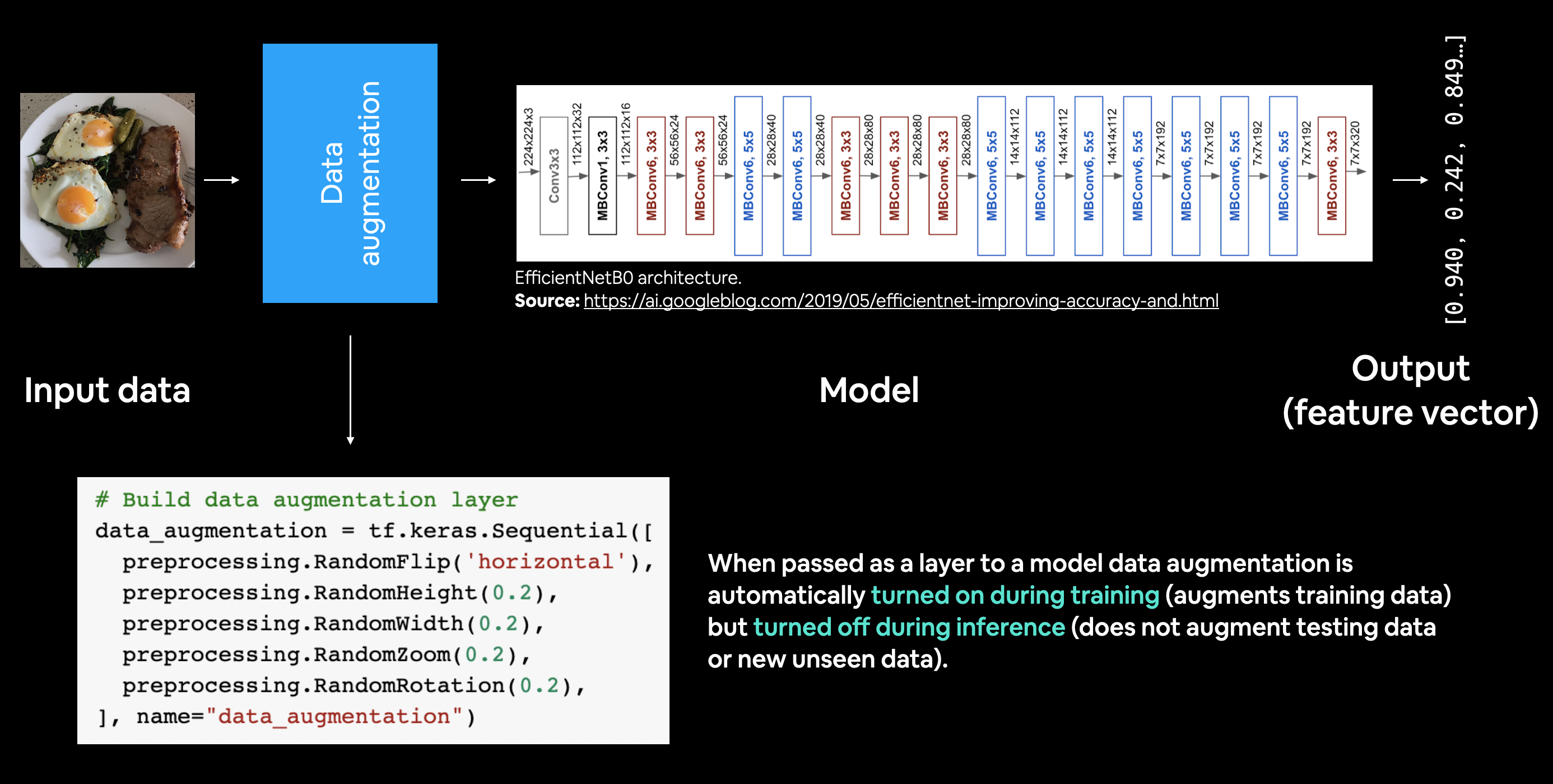 Example of using data augmentation as the first layer within a model (EfficientNetB0).
📚 Resource: For more information on different methods of data augmentation, check out the the TensorFlow data augmentation guide.
To use data augmentation right within our model we'll create a Keras Sequential model consisting of only data preprocessing layers, we can then use this Sequential model within another Functional model.
If that sounds confusing, it'll make sense once we create it in code.
The data augmentation transformations we're going to use are:
tf.keras.layers.RandomFlip- flips image on horizontal or vertical axis.tf.keras.layersRandomRotation- randomly rotates image by a specified amount.tf.keras.layers.RandomZoom- randomly zooms into an image by specified amount.tf.keras.layers.RandomHeight- randomly shifts image height by a specified amount.tf.keras.layers.RandomWidth- randomly shifts image width by a specified amount.tf.keras.layers.Rescaling- normalizes the image pixel values to be between 0 and 1, this is worth mentioning because it is required for some image models but since we're usingtf.keras.applications.efficientnet_v2.EfficientNetV2B0, it's not required (the model pretrained model implements rescaling itself).
There are more option but these will do for now.
import tensorflow as tf
from tensorflow import keras
from tensorflow.keras import layers
# from tensorflow.keras.layers.experimental import preprocessing

# NEW: Newer versions of TensorFlow (2.10+) can use the tensorflow.keras.layers API directly for data augmentation
data_augmentation = keras.Sequential([
  layers.RandomFlip("horizontal"),
  layers.RandomRotation(0.2),
  layers.RandomZoom(0.2),
  layers.RandomHeight(0.2),
  layers.RandomWidth(0.2),
  # preprocessing.Rescaling(1./255) # keep for ResNet50V2, remove for EfficientNetV2B0
], name ="data_augmentation")

# # UPDATE: Previous versions of TensorFlow (e.g. 2.4 and below used the tensorflow.keras.layers.experimental.processing API)
# # Create a data augmentation stage with horizontal flipping, rotations, zooms
# data_augmentation = keras.Sequential([
#   preprocessing.RandomFlip("horizontal"),
#   preprocessing.RandomRotation(0.2),
#   preprocessing.RandomZoom(0.2),
#   preprocessing.RandomHeight(0.2),
#   preprocessing.RandomWidth(0.2),
#   # preprocessing.Rescaling(1./255) # keep for ResNet50V2, remove for EfficientNetV2B0
# ], name ="data_augmentation")
And that's it! Our data augmentation Sequential model is ready to go. As you'll see shortly, we'll be able to slot this "model" as a layer into our transfer learning model later on.
But before we do that, let's test it out by passing random images through it.
# View a random image
import matplotlib.pyplot as plt
import matplotlib.image as mpimg
import os
import random
target_class = random.choice(train_data_1_percent.class_names) # choose a random class
target_dir = "10_food_classes_1_percent/train/" + target_class # create the target directory
random_image = random.choice(os.listdir(target_dir)) # choose a random image from target directory
random_image_path = target_dir + "/" + random_image # create the choosen random image path
img = mpimg.imread(random_image_path) # read in the chosen target image
plt.imshow(img) # plot the target image
plt.title(f"Original random image from class: {target_class}")
plt.axis(False); # turn off the axes

# Augment the image
augmented_img = data_augmentation(tf.expand_dims(img, axis=0)) # data augmentation model requires shape (None, height, width, 3)
plt.figure()
plt.imshow(tf.squeeze(augmented_img)/255.) # requires normalization after augmentation
plt.title(f"Augmented random image from class: {target_class}")
plt.axis(False);


Run the cell above a few times and you can see the different random augmentations on different classes of images. Because we're going to add the data augmentation model as a layer in our upcoming transfer learning model, it'll apply these kind of random augmentations to each of the training images which passes through it.
Doing this will make our training dataset a little more varied. You can think of it as if you were taking a photo of food in real-life, not all of the images are going to be perfect, some of them are going to be orientated in strange ways. These are the kind of images we want our model to be able to handle.
Speaking of model, let's build one with the Functional API. We'll run through all of the same steps as before except for one difference, we'll add our data augmentation Sequential model as a layer immediately after the input layer.
Model 1: Feature extraction transfer learning on 1% of the data with data augmentation
# Setup input shape and base model, freezing the base model layers
input_shape = (224, 224, 3)
base_model = tf.keras.applications.efficientnet_v2.EfficientNetV2B0(include_top=False)
base_model.trainable = False

# Create input layer
inputs = layers.Input(shape=input_shape, name="input_layer")

# Add in data augmentation Sequential model as a layer
x = data_augmentation(inputs)

# Give base_model inputs (after augmentation) and don't train it
x = base_model(x, training=False)

# Pool output features of base model
x = layers.GlobalAveragePooling2D(name="global_average_pooling_layer")(x)

# Put a dense layer on as the output
outputs = layers.Dense(10, activation="softmax", name="output_layer")(x)

# Make a model with inputs and outputs
model_1 = keras.Model(inputs, outputs)

# Compile the model
model_1.compile(loss="categorical_crossentropy",
              optimizer=tf.keras.optimizers.Adam(),
              metrics=["accuracy"])

# Fit the model
history_1_percent = model_1.fit(train_data_1_percent,
                    epochs=5,
                    steps_per_epoch=len(train_data_1_percent),
                    validation_data=test_data,
                    validation_steps=int(0.25* len(test_data)), # validate for less steps
                    # Track model training logs
                    callbacks=[create_tensorboard_callback("transfer_learning", "1_percent_data_aug")])
Saving TensorBoard log files to: transfer_learning/1_percent_data_aug/20230818-014045
Epoch 1/5
3/3 [==============================] - 12s 2s/step - loss: 2.3484 - accuracy: 0.1000 - val_loss: 2.1935 - val_accuracy: 0.1908
Epoch 2/5
3/3 [==============================] - 2s 965ms/step - loss: 2.1591 - accuracy: 0.2000 - val_loss: 2.1027 - val_accuracy: 0.2418
Epoch 3/5
3/3 [==============================] - 2s 894ms/step - loss: 1.9803 - accuracy: 0.3571 - val_loss: 2.0100 - val_accuracy: 0.3076
Epoch 4/5
3/3 [==============================] - 2s 916ms/step - loss: 1.8378 - accuracy: 0.5000 - val_loss: 1.9392 - val_accuracy: 0.3372
Epoch 5/5
3/3 [==============================] - 2s 866ms/step - loss: 1.7660 - accuracy: 0.5429 - val_loss: 1.8595 - val_accuracy: 0.3931
Wow!
How cool is that? Using only 7 training images per class, using transfer learning our model was able to get ~45%+ accuracy on the validation set.
This result is pretty amazing since the original Food-101 paper achieved 50.67% accuracy with all the data, namely, 750 training images per class (note: this metric was across 101 classes, not 10, we'll get to 101 classes soon).
If we check out a summary of our model, we should see the data augmentation layer just after the input layer.
# Check out model summary
model_1.summary()
Model: "model_1"
_________________________________________________________________
 Layer (type)                Output Shape              Param #
=================================================================
 input_layer (InputLayer)    [(None, 224, 224, 3)]     0

 data_augmentation (Sequenti  (None, None, None, 3)    0
 al)

 efficientnetv2-b0 (Function  (None, None, None, 1280)  5919312
 al)

 global_average_pooling_laye  (None, 1280)             0
 r (GlobalAveragePooling2D)

 output_layer (Dense)        (None, 10)                12810

=================================================================
Total params: 5,932,122
Trainable params: 12,810
Non-trainable params: 5,919,312
_________________________________________________________________
There it is. We've now got data augmentation built right into the our model. This means if we saved it and reloaded it somewhere else, the data augmentation layers would come with it.
The important thing to remember is data augmentation only runs during training. So if we were to evaluate or use our model for inference (predicting the class of an image) the data augmentation layers will be automatically turned off.
To see this in action, let's evaluate our model on the test data.
# Evaluate on the test data
results_1_percent_data_aug = model_1.evaluate(test_data)
results_1_percent_data_aug
79/79 [==============================] - 3s 36ms/step - loss: 1.8197 - accuracy: 0.4188
[1.819704294204712, 0.4187999963760376]
The results here may be slightly better/worse than the log outputs of our model during training because during training we only evaluate our model on 25% of the test data using the line validation_steps=int(0.25 * len(test_data)). Doing this speeds up our epochs but still gives us enough of an idea of how our model is going.
Let's stay consistent and check out our model's loss curves.
# How does the model go with a data augmentation layer with 1% of data
plot_loss_curves(history_1_percent)


It looks like the metrics on both datasets would improve if we kept training for more epochs. But we'll leave that for now, we've got more experiments to do!
Model 2: Feature extraction transfer learning with 10% of data and data augmentation
Alright, we've tested 1% of the training data with data augmentation, how about we try 10% of the data with data augmentation?
But wait...
🤔 Question: How do you know what experiments to run?
Great question.
The truth here is you often won't. Machine learning is still a very experimental practice. It's only after trying a fair few things that you'll start to develop an intuition of what to try.
My advice is to follow your curiosity as tenaciously as possible. If you feel like you want to try something, write the code for it and run it. See how it goes. The worst thing that'll happen is you'll figure out what doesn't work, the most valuable kind of knowledge.
From a practical standpoint, as we've talked about before, you'll want to reduce the amount of time between your initial experiments as much as possible. In other words, run a plethora of smaller experiments, using less data and less training iterations before you find something promising and then scale it up.
In the theme of scale, let's scale our 1% training data augmentation experiment up to 10% training data augmentation. That sentence doesn't really make sense but you get what I mean.
We're going to run through the exact same steps as the previous model, the only difference being using 10% of the training data instead of 1%.
# Get 10% of the data of the 10 classes (uncomment if you haven't gotten "10_food_classes_10_percent.zip" already)
# !wget https://storage.googleapis.com/ztm_tf_course/food_vision/10_food_classes_10_percent.zip
# unzip_data("10_food_classes_10_percent.zip")

train_dir_10_percent = "10_food_classes_10_percent/train/"
test_dir = "10_food_classes_10_percent/test/"
Data downloaded. Let's create the dataloaders.
# Setup data inputs
import tensorflow as tf
IMG_SIZE = (224, 224)
train_data_10_percent = tf.keras.preprocessing.image_dataset_from_directory(train_dir_10_percent,
                                                                            label_mode="categorical",
                                                                            image_size=IMG_SIZE)
# Note: the test data is the same as the previous experiment, we could
# skip creating this, but we'll leave this here to practice.
test_data = tf.keras.preprocessing.image_dataset_from_directory(test_dir,
                                                                label_mode="categorical",
                                                                image_size=IMG_SIZE)
Found 750 files belonging to 10 classes.
Found 2500 files belonging to 10 classes.
Awesome!
We've got 10x more images to work with, 75 per class instead of 7 per class.
Let's build a model with data augmentation built in. We could reuse the data augmentation Sequential model we created before but we'll recreate it to practice.
# Create a functional model with data augmentation
import tensorflow as tf
from tensorflow.keras import layers
from tensorflow.keras.models import Sequential
# from tensorflow.keras.layers.experimental import preprocessing # OLD

# NEW: Newer versions of TensorFlow (2.10+) can use the tensorflow.keras.layers API directly for data augmentation
data_augmentation = keras.Sequential([
  layers.RandomFlip("horizontal"),
  layers.RandomRotation(0.2),
  layers.RandomZoom(0.2),
  layers.RandomHeight(0.2),
  layers.RandomWidth(0.2),
  # preprocessing.Rescaling(1./255) # keep for ResNet50V2, remove for EfficientNet
], name ="data_augmentation")

## OLD
# # Build data augmentation layer
# data_augmentation = Sequential([
#   preprocessing.RandomFlip('horizontal'),
#   preprocessing.RandomHeight(0.2),
#   preprocessing.RandomWidth(0.2),
#   preprocessing.RandomZoom(0.2),
#   preprocessing.RandomRotation(0.2),
#   # preprocessing.Rescaling(1./255) # keep for ResNet50V2, remove for EfficientNet
# ], name="data_augmentation")

# Setup the input shape to our model
input_shape = (224, 224, 3)

# Create a frozen base model
# base_model = tf.keras.applications.EfficientNetB0(include_top=False)
base_model = tf.keras.applications.efficientnet_v2.EfficientNetV2B0(include_top=False)
base_model.trainable = False

# Create input and output layers
inputs = layers.Input(shape=input_shape, name="input_layer") # create input layer
x = data_augmentation(inputs) # augment our training images
x = base_model(x, training=False) # pass augmented images to base model but keep it in inference mode, so batchnorm layers don't get updated: https://keras.io/guides/transfer_learning/#build-a-model
x = layers.GlobalAveragePooling2D(name="global_average_pooling_layer")(x)
outputs = layers.Dense(10, activation="softmax", name="output_layer")(x)
model_2 = tf.keras.Model(inputs, outputs)

# Compile
model_2.compile(loss="categorical_crossentropy",
              optimizer=tf.keras.optimizers.Adam(learning_rate=0.001), # use Adam optimizer with base learning rate
              metrics=["accuracy"])
To save time for later (when we want to perform multiple experiments with model_2), let's put the code above into a function we can resuse.
def create_base_model(input_shape: tuple[int, int, int] = (224, 224, 3),
                      output_shape: int = 10,
                      learning_rate: float = 0.001,
                      training: bool = False) -> tf.keras.Model:
    """
    Create a model based on EfficientNetV2B0 with built-in data augmentation.

    Parameters:
    - input_shape (tuple): Expected shape of input images. Default is (224, 224, 3).
    - output_shape (int): Number of classes for the output layer. Default is 10.
    - learning_rate (float): Learning rate for the Adam optimizer. Default is 0.001.
    - training (bool): Whether the base model is trainable. Default is False.

    Returns:
    - tf.keras.Model: The compiled model with specified input and output settings.
    """

    # Create base model
    base_model = tf.keras.applications.efficientnet_v2.EfficientNetV2B0(include_top=False)
    base_model.trainable = training

    # Setup model input and outputs with data augmentation built-in
    inputs = layers.Input(shape=input_shape, name="input_layer")
    x = data_augmentation(inputs)
    x = base_model(x, training=False)  # pass augmented images to base model but keep it in inference mode
    x = layers.GlobalAveragePooling2D(name="global_average_pooling_layer")(x)
    outputs = layers.Dense(units=output_shape, activation="softmax", name="output_layer")(x)
    model = tf.keras.Model(inputs, outputs)

    # Compile model
    model.compile(loss="categorical_crossentropy",
                  optimizer=tf.keras.optimizers.Adam(learning_rate=learning_rate),
                  metrics=["accuracy"])

    return model

# Create an instance of model_2 with our new function
model_2 = create_base_model()
Creating a ModelCheckpoint callback
Our model is compiled and ready to be fit, so why haven't we fit it yet?
Well, for this experiment we're going to introduce a new callback, the ModelCheckpoint callback.
The ModelCheckpoint callback gives you the ability to save your model, as a whole in the SavedModel format or the weights (patterns) only to a specified directory as it trains.
This is helpful if you think your model is going to be training for a long time and you want to make backups of it as it trains. It also means if you think your model could benefit from being trained for longer, you can reload it from a specific checkpoint and continue training from there.
For example, say you fit a feature extraction transfer learning model for 5 epochs and you check the training curves and see it was still improving and you want to see if fine-tuning for another 5 epochs could help, you can load the checkpoint, unfreeze some (or all) of the base model layers and then continue training.
In fact, that's exactly what we're going to do.
But first, let's create a ModelCheckpoint callback. To do so, we have to specifcy a directory we'd like to save to.
# Setup checkpoint path
checkpoint_path = "ten_percent_model_checkpoints_weights/checkpoint.ckpt" # note: remember saving directly to Colab is temporary

# Create a ModelCheckpoint callback that saves the model's weights only
checkpoint_callback = tf.keras.callbacks.ModelCheckpoint(filepath=checkpoint_path,
                                                         save_weights_only=True, # set to False to save the entire model
                                                         save_best_only=True, # save only the best model weights instead of a model every epoch
                                                         save_freq="epoch", # save every epoch
                                                         verbose=1)
🤔 Question: What's the difference between saving the entire model (SavedModel format) and saving the weights only?
The SavedModel format saves a model's architecture, weights and training configuration all in one folder. It makes it very easy to reload your model exactly how it is elsewhere. However, if you do not want to share all of these details with others, you may want to save and share the weights only (these will just be large tensors of non-human interpretable numbers). If disk space is an issue, saving the weights only is faster and takes up less space than saving the whole model.
Time to fit the model.
Because we're going to be fine-tuning it later, we'll create a variable initial_epochs and set it to 5 to use later.
We'll also add in our checkpoint_callback in our list of callbacks.
# Fit the model saving checkpoints every epoch
initial_epochs = 5
history_10_percent_data_aug = model_2.fit(train_data_10_percent,
                                          epochs=initial_epochs,
                                          validation_data=test_data,
                                          validation_steps=int(0.25 * len(test_data)), # do less steps per validation (quicker)
                                          callbacks=[create_tensorboard_callback("transfer_learning", "10_percent_data_aug"),
                                                     checkpoint_callback])
Saving TensorBoard log files to: transfer_learning/10_percent_data_aug/20230818-014119
Epoch 1/5
24/24 [==============================] - ETA: 0s - loss: 2.0057 - accuracy: 0.3360
Epoch 1: val_loss improved from inf to 1.50455, saving model to ten_percent_model_checkpoints_weights/checkpoint.ckpt
24/24 [==============================] - 18s 411ms/step - loss: 2.0057 - accuracy: 0.3360 - val_loss: 1.5045 - val_accuracy: 0.6332
Epoch 2/5
24/24 [==============================] - ETA: 0s - loss: 1.3970 - accuracy: 0.6413
Epoch 2: val_loss improved from 1.50455 to 1.04085, saving model to ten_percent_model_checkpoints_weights/checkpoint.ckpt
24/24 [==============================] - 7s 291ms/step - loss: 1.3970 - accuracy: 0.6413 - val_loss: 1.0408 - val_accuracy: 0.7615
Epoch 3/5
24/24 [==============================] - ETA: 0s - loss: 1.1097 - accuracy: 0.7253
Epoch 3: val_loss improved from 1.04085 to 0.86102, saving model to ten_percent_model_checkpoints_weights/checkpoint.ckpt
24/24 [==============================] - 7s 285ms/step - loss: 1.1097 - accuracy: 0.7253 - val_loss: 0.8610 - val_accuracy: 0.7895
Epoch 4/5
24/24 [==============================] - ETA: 0s - loss: 0.9359 - accuracy: 0.7707
Epoch 4: val_loss improved from 0.86102 to 0.72648, saving model to ten_percent_model_checkpoints_weights/checkpoint.ckpt
24/24 [==============================] - 6s 247ms/step - loss: 0.9359 - accuracy: 0.7707 - val_loss: 0.7265 - val_accuracy: 0.8306
Epoch 5/5
24/24 [==============================] - ETA: 0s - loss: 0.8332 - accuracy: 0.7840
Epoch 5: val_loss improved from 0.72648 to 0.68383, saving model to ten_percent_model_checkpoints_weights/checkpoint.ckpt
24/24 [==============================] - 6s 249ms/step - loss: 0.8332 - accuracy: 0.7840 - val_loss: 0.6838 - val_accuracy: 0.8240
Would you look at that! Looks like our ModelCheckpoint callback worked and our model saved its weights every epoch without too much overhead (saving the whole model takes longer than just the weights).
Let's evaluate our model and check its loss curves.
# Evaluate on the test data
results_10_percent_data_aug = model_2.evaluate(test_data)
results_10_percent_data_aug
79/79 [==============================] - 3s 34ms/step - loss: 0.6795 - accuracy: 0.8216
[0.6794611215591431, 0.8216000199317932]
# Plot model loss curves
plot_loss_curves(history_10_percent_data_aug)


Looking at these, our model's performance with 10% of the data and data augmentation isn't as good as the model with 10% of the data without data augmentation (see model_0 results above), however the curves are trending in the right direction, meaning if we decided to train for longer, its metrics would likely improve.
Since we checkpointed (is that a word?) our model's weights, we might as well see what it's like to load it back in. We'll be able to test if it saved correctly by evaluting it on the test data.
To load saved model weights you can use the the load_weights() method, passing it the path where your saved weights are stored.
# Load in saved model weights and evaluate model
model_2.load_weights(checkpoint_path)
loaded_weights_model_results = model_2.evaluate(test_data)
79/79 [==============================] - 3s 38ms/step - loss: 0.6795 - accuracy: 0.8216
Now let's compare the results of our previously trained model and the loaded model. These results should very close if not exactly the same. The reason for minor differences comes down to the precision level of numbers calculated.
# If the results from our native model and the loaded weights are the same, this should output True
results_10_percent_data_aug == loaded_weights_model_results
True
If the above cell doesn't output True, it's because the numbers are close but not the exact same (due to how computers store numbers with degrees of precision).
However, they should be very close...
import numpy as np
# Check to see if loaded model results are very close to native model results (should output True)
np.isclose(np.array(results_10_percent_data_aug), np.array(loaded_weights_model_results))
array([ True, True])
# Check the difference between the two results (small values)
print(np.array(results_10_percent_data_aug) - np.array(loaded_weights_model_results))
[0. 0.]
Model 3: Fine-tuning an existing model on 10% of the data
 High-level example of fine-tuning an EfficientNet model. Bottom layers (layers closer to the input data) stay frozen where as top layers (layers closer to the output data) are updated during training.
So far our saved model has been trained using feature extraction transfer learning for 5 epochs on 10% of the training data and data augmentation.
This means all of the layers in the base model (EfficientNetV2B0) were frozen during training.
For our next experiment we're going to switch to fine-tuning transfer learning. This means we'll be using the same base model except we'll be unfreezing some of its layers (ones closest to the top) and running the model for a few more epochs.
The idea with fine-tuning is to start customizing the pre-trained model more to our own data.
🔑 Note: Fine-tuning usually works best after training a feature extraction model for a few epochs and with large amounts of data. For more on this, check out Keras' guide on Transfer learning & fine-tuning.
We've verified our loaded model's performance, let's check out its layers.
# Layers in loaded model
model_2.layers
[<keras.engine.input_layer.InputLayer at 0x7c62e86157b0>,
 <keras.engine.sequential.Sequential at 0x7c62e8188280>,
 <keras.engine.functional.Functional at 0x7c62a3daecb0>,
 <keras.layers.pooling.global_average_pooling2d.GlobalAveragePooling2D at 0x7c62a3c0a890>,
 <keras.layers.core.dense.Dense at 0x7c62a3ddbf70>]
How about we check their names, numbers and if they're trainable?
for layer_number, layer in enumerate(model_2.layers):
  print(f"Layer number: {layer_number} | Layer name: {layer.name} | Layer type: {layer} | Trainable? {layer.trainable}")
Layer number: 0 | Layer name: input_layer | Layer type: <keras.engine.input_layer.InputLayer object at 0x7c62e86157b0> | Trainable? True
Layer number: 1 | Layer name: data_augmentation | Layer type: <keras.engine.sequential.Sequential object at 0x7c62e8188280> | Trainable? True
Layer number: 2 | Layer name: efficientnetv2-b0 | Layer type: <keras.engine.functional.Functional object at 0x7c62a3daecb0> | Trainable? False
Layer number: 3 | Layer name: global_average_pooling_layer | Layer type: <keras.layers.pooling.global_average_pooling2d.GlobalAveragePooling2D object at 0x7c62a3c0a890> | Trainable? True
Layer number: 4 | Layer name: output_layer | Layer type: <keras.layers.core.dense.Dense object at 0x7c62a3ddbf70> | Trainable? True
Looking good.
We've got an input layer, a Sequential layer (the data augmentation model), a Functional layer (EfficientNetV2B0), a pooling layer and a Dense layer (the output layer).
How about a summary?
model_2.summary()
Model: "model_3"
_________________________________________________________________
 Layer (type)                Output Shape              Param #
=================================================================
 input_layer (InputLayer)    [(None, 224, 224, 3)]     0

 data_augmentation (Sequenti  (None, None, None, 3)    0
 al)

 efficientnetv2-b0 (Function  (None, None, None, 1280)  5919312
 al)

 global_average_pooling_laye  (None, 1280)             0
 r (GlobalAveragePooling2D)

 output_layer (Dense)        (None, 10)                12810

=================================================================
Total params: 5,932,122
Trainable params: 12,810
Non-trainable params: 5,919,312
_________________________________________________________________
Alright, it looks like all of the layers in the efficientnetv2-b0 layer are frozen. We can confirm this using the trainable_variables attribute.
Note: The layers of
base_model(ourefficientnetv2-b0feature extractor) ofmodel_2is accessible by referencingmodel_2.layers[2].
# Access the base_model layers of model_2
model_2_base_model = model_2.layers[2]
model_2_base_model.name
'efficientnetv2-b0'
# How many layers are trainable in our model_2_base_model?
print(len(model_2_base_model.trainable_variables)) # layer at index 2 is the EfficientNetV2B0 layer (the base model)
0
We can even check layer by layer to see if the they're trainable.
To access the layers in model_2_base_model, we can use the layers attribute.
# Check which layers are tuneable (trainable)
for layer_number, layer in enumerate(model_2_base_model.layers):
  print(layer_number, layer.name, layer.trainable)
0 input_4 False
1 rescaling_3 False
2 normalization_3 False
3 stem_conv False
4 stem_bn False
5 stem_activation False
6 block1a_project_conv False
7 block1a_project_bn False
8 block1a_project_activation False
9 block2a_expand_conv False
10 block2a_expand_bn False
11 block2a_expand_activation False
12 block2a_project_conv False
13 block2a_project_bn False
14 block2b_expand_conv False
15 block2b_expand_bn False
16 block2b_expand_activation False
17 block2b_project_conv False
18 block2b_project_bn False
19 block2b_drop False
20 block2b_add False
21 block3a_expand_conv False
22 block3a_expand_bn False
23 block3a_expand_activation False
24 block3a_project_conv False
25 block3a_project_bn False
26 block3b_expand_conv False
27 block3b_expand_bn False
28 block3b_expand_activation False
29 block3b_project_conv False
30 block3b_project_bn False
31 block3b_drop False
32 block3b_add False
33 block4a_expand_conv False
34 block4a_expand_bn False
35 block4a_expand_activation False
36 block4a_dwconv2 False
37 block4a_bn False
38 block4a_activation False
39 block4a_se_squeeze False
40 block4a_se_reshape False
41 block4a_se_reduce False
42 block4a_se_expand False
43 block4a_se_excite False
44 block4a_project_conv False
45 block4a_project_bn False
46 block4b_expand_conv False
47 block4b_expand_bn False
48 block4b_expand_activation False
49 block4b_dwconv2 False
50 block4b_bn False
51 block4b_activation False
52 block4b_se_squeeze False
53 block4b_se_reshape False
54 block4b_se_reduce False
55 block4b_se_expand False
56 block4b_se_excite False
57 block4b_project_conv False
58 block4b_project_bn False
59 block4b_drop False
60 block4b_add False
61 block4c_expand_conv False
62 block4c_expand_bn False
63 block4c_expand_activation False
64 block4c_dwconv2 False
65 block4c_bn False
66 block4c_activation False
67 block4c_se_squeeze False
68 block4c_se_reshape False
69 block4c_se_reduce False
70 block4c_se_expand False
71 block4c_se_excite False
72 block4c_project_conv False
73 block4c_project_bn False
74 block4c_drop False
75 block4c_add False
76 block5a_expand_conv False
77 block5a_expand_bn False
78 block5a_expand_activation False
79 block5a_dwconv2 False
80 block5a_bn False
81 block5a_activation False
82 block5a_se_squeeze False
83 block5a_se_reshape False
84 block5a_se_reduce False
85 block5a_se_expand False
86 block5a_se_excite False
87 block5a_project_conv False
88 block5a_project_bn False
89 block5b_expand_conv False
90 block5b_expand_bn False
91 block5b_expand_activation False
92 block5b_dwconv2 False
93 block5b_bn False
94 block5b_activation False
95 block5b_se_squeeze False
96 block5b_se_reshape False
97 block5b_se_reduce False
98 block5b_se_expand False
99 block5b_se_excite False
100 block5b_project_conv False
101 block5b_project_bn False
102 block5b_drop False
103 block5b_add False
104 block5c_expand_conv False
105 block5c_expand_bn False
106 block5c_expand_activation False
107 block5c_dwconv2 False
108 block5c_bn False
109 block5c_activation False
110 block5c_se_squeeze False
111 block5c_se_reshape False
112 block5c_se_reduce False
113 block5c_se_expand False
114 block5c_se_excite False
115 block5c_project_conv False
116 block5c_project_bn False
117 block5c_drop False
118 block5c_add False
119 block5d_expand_conv False
120 block5d_expand_bn False
121 block5d_expand_activation False
122 block5d_dwconv2 False
123 block5d_bn False
124 block5d_activation False
125 block5d_se_squeeze False
126 block5d_se_reshape False
127 block5d_se_reduce False
128 block5d_se_expand False
129 block5d_se_excite False
130 block5d_project_conv False
131 block5d_project_bn False
132 block5d_drop False
133 block5d_add False
134 block5e_expand_conv False
135 block5e_expand_bn False
136 block5e_expand_activation False
137 block5e_dwconv2 False
138 block5e_bn False
139 block5e_activation False
140 block5e_se_squeeze False
141 block5e_se_reshape False
142 block5e_se_reduce False
143 block5e_se_expand False
144 block5e_se_excite False
145 block5e_project_conv False
146 block5e_project_bn False
147 block5e_drop False
148 block5e_add False
149 block6a_expand_conv False
150 block6a_expand_bn False
151 block6a_expand_activation False
152 block6a_dwconv2 False
153 block6a_bn False
154 block6a_activation False
155 block6a_se_squeeze False
156 block6a_se_reshape False
157 block6a_se_reduce False
158 block6a_se_expand False
159 block6a_se_excite False
160 block6a_project_conv False
161 block6a_project_bn False
162 block6b_expand_conv False
163 block6b_expand_bn False
164 block6b_expand_activation False
165 block6b_dwconv2 False
166 block6b_bn False
167 block6b_activation False
168 block6b_se_squeeze False
169 block6b_se_reshape False
170 block6b_se_reduce False
171 block6b_se_expand False
172 block6b_se_excite False
173 block6b_project_conv False
174 block6b_project_bn False
175 block6b_drop False
176 block6b_add False
177 block6c_expand_conv False
178 block6c_expand_bn False
179 block6c_expand_activation False
180 block6c_dwconv2 False
181 block6c_bn False
182 block6c_activation False
183 block6c_se_squeeze False
184 block6c_se_reshape False
185 block6c_se_reduce False
186 block6c_se_expand False
187 block6c_se_excite False
188 block6c_project_conv False
189 block6c_project_bn False
190 block6c_drop False
191 block6c_add False
192 block6d_expand_conv False
193 block6d_expand_bn False
194 block6d_expand_activation False
195 block6d_dwconv2 False
196 block6d_bn False
197 block6d_activation False
198 block6d_se_squeeze False
199 block6d_se_reshape False
200 block6d_se_reduce False
201 block6d_se_expand False
202 block6d_se_excite False
203 block6d_project_conv False
204 block6d_project_bn False
205 block6d_drop False
206 block6d_add False
207 block6e_expand_conv False
208 block6e_expand_bn False
209 block6e_expand_activation False
210 block6e_dwconv2 False
211 block6e_bn False
212 block6e_activation False
213 block6e_se_squeeze False
214 block6e_se_reshape False
215 block6e_se_reduce False
216 block6e_se_expand False
217 block6e_se_excite False
218 block6e_project_conv False
219 block6e_project_bn False
220 block6e_drop False
221 block6e_add False
222 block6f_expand_conv False
223 block6f_expand_bn False
224 block6f_expand_activation False
225 block6f_dwconv2 False
226 block6f_bn False
227 block6f_activation False
228 block6f_se_squeeze False
229 block6f_se_reshape False
230 block6f_se_reduce False
231 block6f_se_expand False
232 block6f_se_excite False
233 block6f_project_conv False
234 block6f_project_bn False
235 block6f_drop False
236 block6f_add False
237 block6g_expand_conv False
238 block6g_expand_bn False
239 block6g_expand_activation False
240 block6g_dwconv2 False
241 block6g_bn False
242 block6g_activation False
243 block6g_se_squeeze False
244 block6g_se_reshape False
245 block6g_se_reduce False
246 block6g_se_expand False
247 block6g_se_excite False
248 block6g_project_conv False
249 block6g_project_bn False
250 block6g_drop False
251 block6g_add False
252 block6h_expand_conv False
253 block6h_expand_bn False
254 block6h_expand_activation False
255 block6h_dwconv2 False
256 block6h_bn False
257 block6h_activation False
258 block6h_se_squeeze False
259 block6h_se_reshape False
260 block6h_se_reduce False
261 block6h_se_expand False
262 block6h_se_excite False
263 block6h_project_conv False
264 block6h_project_bn False
265 block6h_drop False
266 block6h_add False
267 top_conv False
268 top_bn False
269 top_activation False
Beautiful. This is exactly what we're after.
Now to fine-tune the base model to our own data, we're going to unfreeze the top 10 layers and continue training our model for another 5 epochs.
This means all of the base model's layers except for the last 10 will remain frozen and untrainable. And the weights in the remaining unfrozen layers will be updated during training.
Ideally, we should see the model's performance improve.
🤔 Question: How many layers should you unfreeze when training?
There's no set rule for this. You could unfreeze every layer in the pretrained model or you could try unfreezing one layer at a time. Best to experiment with different amounts of unfreezing and fine-tuning to see what happens. Generally, the less data you have, the less layers you want to unfreeze and the more gradually you want to fine-tune.
📖 Resource: The ULMFiT (Universal Language Model Fine-tuning for Text Classification) paper has a great series of experiments on fine-tuning models.
To begin fine-tuning, we'll unfreeze the entire model_2_base_model by setting its trainable attribute to True.
Then we'll refreeze every layer in model_2_base_model except for the last 10 by looping through them and setting their trainable attribute to False.
Finally, we'll recompile the whole model.
# Make all the layers in model_2_base_model trainable
model_2_base_model.trainable = True

# Freeze all layers except for the last 10
for layer in model_2_base_model.layers[:-10]:
  layer.trainable = False

# Recompile the whole model (always recompile after any adjustments to a model)
model_2.compile(loss="categorical_crossentropy",
                optimizer=tf.keras.optimizers.Adam(learning_rate=0.0001), # lr is 10x lower than before for fine-tuning
                metrics=["accuracy"])
Wonderful, now let's check which layers of the pretrained model are trainable.
# Check which layers are tuneable (trainable)
for layer_number, layer in enumerate(model_2_base_model.layers):
  print(layer_number, layer.name, layer.trainable)
0 input_4 False
1 rescaling_3 False
2 normalization_3 False
3 stem_conv False
4 stem_bn False
5 stem_activation False
6 block1a_project_conv False
7 block1a_project_bn False
8 block1a_project_activation False
9 block2a_expand_conv False
10 block2a_expand_bn False
11 block2a_expand_activation False
12 block2a_project_conv False
13 block2a_project_bn False
14 block2b_expand_conv False
15 block2b_expand_bn False
16 block2b_expand_activation False
17 block2b_project_conv False
18 block2b_project_bn False
19 block2b_drop False
20 block2b_add False
21 block3a_expand_conv False
22 block3a_expand_bn False
23 block3a_expand_activation False
24 block3a_project_conv False
25 block3a_project_bn False
26 block3b_expand_conv False
27 block3b_expand_bn False
28 block3b_expand_activation False
29 block3b_project_conv False
30 block3b_project_bn False
31 block3b_drop False
32 block3b_add False
33 block4a_expand_conv False
34 block4a_expand_bn False
35 block4a_expand_activation False
36 block4a_dwconv2 False
37 block4a_bn False
38 block4a_activation False
39 block4a_se_squeeze False
40 block4a_se_reshape False
41 block4a_se_reduce False
42 block4a_se_expand False
43 block4a_se_excite False
44 block4a_project_conv False
45 block4a_project_bn False
46 block4b_expand_conv False
47 block4b_expand_bn False
48 block4b_expand_activation False
49 block4b_dwconv2 False
50 block4b_bn False
51 block4b_activation False
52 block4b_se_squeeze False
53 block4b_se_reshape False
54 block4b_se_reduce False
55 block4b_se_expand False
56 block4b_se_excite False
57 block4b_project_conv False
58 block4b_project_bn False
59 block4b_drop False
60 block4b_add False
61 block4c_expand_conv False
62 block4c_expand_bn False
63 block4c_expand_activation False
64 block4c_dwconv2 False
65 block4c_bn False
66 block4c_activation False
67 block4c_se_squeeze False
68 block4c_se_reshape False
69 block4c_se_reduce False
70 block4c_se_expand False
71 block4c_se_excite False
72 block4c_project_conv False
73 block4c_project_bn False
74 block4c_drop False
75 block4c_add False
76 block5a_expand_conv False
77 block5a_expand_bn False
78 block5a_expand_activation False
79 block5a_dwconv2 False
80 block5a_bn False
81 block5a_activation False
82 block5a_se_squeeze False
83 block5a_se_reshape False
84 block5a_se_reduce False
85 block5a_se_expand False
86 block5a_se_excite False
87 block5a_project_conv False
88 block5a_project_bn False
89 block5b_expand_conv False
90 block5b_expand_bn False
91 block5b_expand_activation False
92 block5b_dwconv2 False
93 block5b_bn False
94 block5b_activation False
95 block5b_se_squeeze False
96 block5b_se_reshape False
97 block5b_se_reduce False
98 block5b_se_expand False
99 block5b_se_excite False
100 block5b_project_conv False
101 block5b_project_bn False
102 block5b_drop False
103 block5b_add False
104 block5c_expand_conv False
105 block5c_expand_bn False
106 block5c_expand_activation False
107 block5c_dwconv2 False
108 block5c_bn False
109 block5c_activation False
110 block5c_se_squeeze False
111 block5c_se_reshape False
112 block5c_se_reduce False
113 block5c_se_expand False
114 block5c_se_excite False
115 block5c_project_conv False
116 block5c_project_bn False
117 block5c_drop False
118 block5c_add False
119 block5d_expand_conv False
120 block5d_expand_bn False
121 block5d_expand_activation False
122 block5d_dwconv2 False
123 block5d_bn False
124 block5d_activation False
125 block5d_se_squeeze False
126 block5d_se_reshape False
127 block5d_se_reduce False
128 block5d_se_expand False
129 block5d_se_excite False
130 block5d_project_conv False
131 block5d_project_bn False
132 block5d_drop False
133 block5d_add False
134 block5e_expand_conv False
135 block5e_expand_bn False
136 block5e_expand_activation False
137 block5e_dwconv2 False
138 block5e_bn False
139 block5e_activation False
140 block5e_se_squeeze False
141 block5e_se_reshape False
142 block5e_se_reduce False
143 block5e_se_expand False
144 block5e_se_excite False
145 block5e_project_conv False
146 block5e_project_bn False
147 block5e_drop False
148 block5e_add False
149 block6a_expand_conv False
150 block6a_expand_bn False
151 block6a_expand_activation False
152 block6a_dwconv2 False
153 block6a_bn False
154 block6a_activation False
155 block6a_se_squeeze False
156 block6a_se_reshape False
157 block6a_se_reduce False
158 block6a_se_expand False
159 block6a_se_excite False
160 block6a_project_conv False
161 block6a_project_bn False
162 block6b_expand_conv False
163 block6b_expand_bn False
164 block6b_expand_activation False
165 block6b_dwconv2 False
166 block6b_bn False
167 block6b_activation False
168 block6b_se_squeeze False
169 block6b_se_reshape False
170 block6b_se_reduce False
171 block6b_se_expand False
172 block6b_se_excite False
173 block6b_project_conv False
174 block6b_project_bn False
175 block6b_drop False
176 block6b_add False
177 block6c_expand_conv False
178 block6c_expand_bn False
179 block6c_expand_activation False
180 block6c_dwconv2 False
181 block6c_bn False
182 block6c_activation False
183 block6c_se_squeeze False
184 block6c_se_reshape False
185 block6c_se_reduce False
186 block6c_se_expand False
187 block6c_se_excite False
188 block6c_project_conv False
189 block6c_project_bn False
190 block6c_drop False
191 block6c_add False
192 block6d_expand_conv False
193 block6d_expand_bn False
194 block6d_expand_activation False
195 block6d_dwconv2 False
196 block6d_bn False
197 block6d_activation False
198 block6d_se_squeeze False
199 block6d_se_reshape False
200 block6d_se_reduce False
201 block6d_se_expand False
202 block6d_se_excite False
203 block6d_project_conv False
204 block6d_project_bn False
205 block6d_drop False
206 block6d_add False
207 block6e_expand_conv False
208 block6e_expand_bn False
209 block6e_expand_activation False
210 block6e_dwconv2 False
211 block6e_bn False
212 block6e_activation False
213 block6e_se_squeeze False
214 block6e_se_reshape False
215 block6e_se_reduce False
216 block6e_se_expand False
217 block6e_se_excite False
218 block6e_project_conv False
219 block6e_project_bn False
220 block6e_drop False
221 block6e_add False
222 block6f_expand_conv False
223 block6f_expand_bn False
224 block6f_expand_activation False
225 block6f_dwconv2 False
226 block6f_bn False
227 block6f_activation False
228 block6f_se_squeeze False
229 block6f_se_reshape False
230 block6f_se_reduce False
231 block6f_se_expand False
232 block6f_se_excite False
233 block6f_project_conv False
234 block6f_project_bn False
235 block6f_drop False
236 block6f_add False
237 block6g_expand_conv False
238 block6g_expand_bn False
239 block6g_expand_activation False
240 block6g_dwconv2 False
241 block6g_bn False
242 block6g_activation False
243 block6g_se_squeeze False
244 block6g_se_reshape False
245 block6g_se_reduce False
246 block6g_se_expand False
247 block6g_se_excite False
248 block6g_project_conv False
249 block6g_project_bn False
250 block6g_drop False
251 block6g_add False
252 block6h_expand_conv False
253 block6h_expand_bn False
254 block6h_expand_activation False
255 block6h_dwconv2 False
256 block6h_bn False
257 block6h_activation False
258 block6h_se_squeeze False
259 block6h_se_reshape False
260 block6h_se_reduce True
261 block6h_se_expand True
262 block6h_se_excite True
263 block6h_project_conv True
264 block6h_project_bn True
265 block6h_drop True
266 block6h_add True
267 top_conv True
268 top_bn True
269 top_activation True
Nice! It seems all layers except for the last 10 are frozen and untrainable. This means only the last 10 layers of the base model along with the output layer will have their weights updated during training.
🤔 Question: Why did we recompile the model?
Every time you make a change to your models, you need to recompile them.
In our case, we're using the exact same loss, optimizer and metrics as before, except this time the learning rate for our optimizer will be 10x smaller than before (0.0001 instead of Adam's default of 0.001).
We do this so the model doesn't try to overwrite the existing weights in the pretrained model too fast. In other words, we want learning to be more gradual.
🔑 Note: There's no set standard for setting the learning rate during fine-tuning, though reductions of 2.6x-10x+ seem to work well in practice.
How many trainable variables do we have now?
print(len(model_2.trainable_variables))
12
Wonderful, it looks like our model has a total of 12 trainable variables, the last 10 layers of the base model and the weight and bias parameters of the Dense output layer.
Time to fine-tune!
We're going to continue training on from where our previous model finished. Since it trained for 5 epochs, our fine-tuning will begin on the epoch 5 and continue for another 5 epochs.
To do this, we can use the initial_epoch parameter of the fit() method. We'll pass it the last epoch of the previous model's training history (history_10_percent_data_aug.epoch[-1]).
# Fine tune for another 5 epochs
fine_tune_epochs = initial_epochs + 5

# Refit the model (same as model_2 except with more trainable layers)
history_fine_10_percent_data_aug = model_2.fit(train_data_10_percent,
                                               epochs=fine_tune_epochs,
                                               validation_data=test_data,
                                               initial_epoch=history_10_percent_data_aug.epoch[-1], # start from previous last epoch
                                               validation_steps=int(0.25 * len(test_data)),
                                               callbacks=[create_tensorboard_callback("transfer_learning", "10_percent_fine_tune_last_10")]) # name experiment appropriately
Saving TensorBoard log files to: transfer_learning/10_percent_fine_tune_last_10/20230818-014212
Epoch 5/10
24/24 [==============================] - 19s 333ms/step - loss: 0.7145 - accuracy: 0.8080 - val_loss: 0.5455 - val_accuracy: 0.8355
Epoch 6/10
24/24 [==============================] - 6s 228ms/step - loss: 0.6243 - accuracy: 0.8133 - val_loss: 0.5008 - val_accuracy: 0.8372
Epoch 7/10
24/24 [==============================] - 5s 199ms/step - loss: 0.5388 - accuracy: 0.8333 - val_loss: 0.4581 - val_accuracy: 0.8520
Epoch 8/10
24/24 [==============================] - 5s 215ms/step - loss: 0.5132 - accuracy: 0.8427 - val_loss: 0.4846 - val_accuracy: 0.8487
Epoch 9/10
24/24 [==============================] - 5s 191ms/step - loss: 0.4753 - accuracy: 0.8467 - val_loss: 0.4536 - val_accuracy: 0.8569
Epoch 10/10
24/24 [==============================] - 6s 225ms/step - loss: 0.4245 - accuracy: 0.8653 - val_loss: 0.4656 - val_accuracy: 0.8470
🔑 Note: Fine-tuning usually takes far longer per epoch than feature extraction (due to updating more weights throughout a network).
Ho ho, looks like our model has gained a few percentage points of accuracy! Let's evalaute it.
# Evaluate the model on the test data
results_fine_tune_10_percent = model_2.evaluate(test_data)
79/79 [==============================] - 3s 31ms/step - loss: 0.4526 - accuracy: 0.8504
Remember, the results from evaluating the model might be slightly different to the outputs from training since during training we only evaluate on 25% of the test data.
Alright, we need a way to evaluate our model's performance before and after fine-tuning. How about we write a function to compare the before and after?
def compare_historys(original_history, new_history, initial_epochs=5):
    """
    Compares two model history objects.
    """
    # Get original history measurements
    acc = original_history.history["accuracy"]
    loss = original_history.history["loss"]

    print(len(acc))

    val_acc = original_history.history["val_accuracy"]
    val_loss = original_history.history["val_loss"]

    # Combine original history with new history
    total_acc = acc + new_history.history["accuracy"]
    total_loss = loss + new_history.history["loss"]

    total_val_acc = val_acc + new_history.history["val_accuracy"]
    total_val_loss = val_loss + new_history.history["val_loss"]

    print(len(total_acc))
    print(total_acc)

    # Make plots
    plt.figure(figsize=(8, 8))
    plt.subplot(2, 1, 1)
    plt.plot(total_acc, label='Training Accuracy')
    plt.plot(total_val_acc, label='Validation Accuracy')
    plt.plot([initial_epochs-1, initial_epochs-1],
              plt.ylim(), label='Start Fine Tuning') # reshift plot around epochs
    plt.legend(loc='lower right')
    plt.title('Training and Validation Accuracy')

    plt.subplot(2, 1, 2)
    plt.plot(total_loss, label='Training Loss')
    plt.plot(total_val_loss, label='Validation Loss')
    plt.plot([initial_epochs-1, initial_epochs-1],
              plt.ylim(), label='Start Fine Tuning') # reshift plot around epochs
    plt.legend(loc='upper right')
    plt.title('Training and Validation Loss')
    plt.xlabel('epoch')
    plt.show()
This is where saving the history variables of our model training comes in handy. Let's see what happened after fine-tuning the last 10 layers of our model.
compare_historys(original_history=history_10_percent_data_aug,
                 new_history=history_fine_10_percent_data_aug,
                 initial_epochs=5)
5
11
[0.335999995470047, 0.6413333415985107, 0.7253333330154419, 0.7706666588783264, 0.7839999794960022, 0.8080000281333923, 0.8133333325386047, 0.8333333134651184, 0.8426666855812073, 0.846666693687439, 0.8653333187103271]

Alright, alright, seems like the curves are heading in the right direction after fine-tuning. But remember, it should be noted that fine-tuning usually works best with larger amounts of data.
Model 4: Fine-tuning an existing model all of the data
Enough talk about how fine-tuning a model usually works with more data, let's try it out.
We'll start by downloading the full version of our 10 food classes dataset.
# Download and unzip 10 classes of data with all images
!wget https://storage.googleapis.com/ztm_tf_course/food_vision/10_food_classes_all_data.zip
unzip_data("10_food_classes_all_data.zip")

# Setup data directories
train_dir = "10_food_classes_all_data/train/"
test_dir = "10_food_classes_all_data/test/"
--2023-08-18 01:43:01--  https://storage.googleapis.com/ztm_tf_course/food_vision/10_food_classes_all_data.zip
Resolving storage.googleapis.com (storage.googleapis.com)... 173.194.202.128, 173.194.203.128, 74.125.199.128, ...
Connecting to storage.googleapis.com (storage.googleapis.com)|173.194.202.128|:443... connected.
HTTP request sent, awaiting response... 200 OK
Length: 519183241 (495M) [application/zip]
Saving to: ‘10_food_classes_all_data.zip’

10_food_classes_all 100%[===================>] 495.13M   148MB/s    in 3.5s

2023-08-18 01:43:04 (143 MB/s) - ‘10_food_classes_all_data.zip’ saved [519183241/519183241]
# How many images are we working with now?
walk_through_dir("10_food_classes_all_data")
There are 2 directories and 0 images in '10_food_classes_all_data'.
There are 10 directories and 0 images in '10_food_classes_all_data/train'.
There are 0 directories and 750 images in '10_food_classes_all_data/train/ramen'.
There are 0 directories and 750 images in '10_food_classes_all_data/train/chicken_curry'.
There are 0 directories and 750 images in '10_food_classes_all_data/train/pizza'.
There are 0 directories and 750 images in '10_food_classes_all_data/train/ice_cream'.
There are 0 directories and 750 images in '10_food_classes_all_data/train/grilled_salmon'.
There are 0 directories and 750 images in '10_food_classes_all_data/train/steak'.
There are 0 directories and 750 images in '10_food_classes_all_data/train/chicken_wings'.
There are 0 directories and 750 images in '10_food_classes_all_data/train/hamburger'.
There are 0 directories and 750 images in '10_food_classes_all_data/train/sushi'.
There are 0 directories and 750 images in '10_food_classes_all_data/train/fried_rice'.
There are 10 directories and 0 images in '10_food_classes_all_data/test'.
There are 0 directories and 250 images in '10_food_classes_all_data/test/ramen'.
There are 0 directories and 250 images in '10_food_classes_all_data/test/chicken_curry'.
There are 0 directories and 250 images in '10_food_classes_all_data/test/pizza'.
There are 0 directories and 250 images in '10_food_classes_all_data/test/ice_cream'.
There are 0 directories and 250 images in '10_food_classes_all_data/test/grilled_salmon'.
There are 0 directories and 250 images in '10_food_classes_all_data/test/steak'.
There are 0 directories and 250 images in '10_food_classes_all_data/test/chicken_wings'.
There are 0 directories and 250 images in '10_food_classes_all_data/test/hamburger'.
There are 0 directories and 250 images in '10_food_classes_all_data/test/sushi'.
There are 0 directories and 250 images in '10_food_classes_all_data/test/fried_rice'.
And now we'll turn the images into tensors datasets.
# Setup data inputs
import tensorflow as tf
IMG_SIZE = (224, 224)
train_data_10_classes_full = tf.keras.preprocessing.image_dataset_from_directory(train_dir,
                                                                                 label_mode="categorical",
                                                                                 image_size=IMG_SIZE)

# Note: this is the same test dataset we've been using for the previous modelling experiments
test_data = tf.keras.preprocessing.image_dataset_from_directory(test_dir,
                                                                label_mode="categorical",
                                                                image_size=IMG_SIZE)
Found 7500 files belonging to 10 classes.
Found 2500 files belonging to 10 classes.
Oh this is looking good. We've got 10x more images in of the training classes to work with.
The test dataset is the same we've been using for our previous experiments.
As it is now, our model_2 has been fine-tuned on 10 percent of the data, so to begin fine-tuning on all of the data and keep our experiments consistent, we need to revert it back to the weights we checkpointed after 5 epochs of feature-extraction.
To demonstrate this, we'll first evaluate the current model_2.
# Evaluate model (this is the fine-tuned 10 percent of data version)
model_2.evaluate(test_data)
79/79 [==============================] - 3s 39ms/step - loss: 0.4526 - accuracy: 0.8504
[0.452595591545105, 0.8503999710083008]
These are the same values as results_fine_tune_10_percent.
results_fine_tune_10_percent
[0.4525955617427826, 0.8503999710083008]
To keep our experiments clean, we'll load a create a new instance of model_2 using our create_base_model() function.
More specifically, we're trying to measure:
- Experiment 3 (previous one) -
model_2with 10 layers fine-tuned for 5 more epochs on 10% of the data. - Experiment 4 (this one) -
model_2with layers fined-tuned for 5 more epochs on 100% on the data.
Importantly, both experiments should use the same test data (to keep evaluation the same).
And they should also start from the same checkpoint (model_2 feature extractor trained for 5 epochs on 10% of the data).
Let's first create new instance of model_2.
# Create a new instance of model_2 for Experiment 4
model_2 = create_base_model(learning_rate=0.0001) # 10x lower learning rate for fine-tuning
And now to make sure it starts at the same checkpoint, we can load the checkpointed weights from checkpoint_path.
# Load previously checkpointed weights
model_2.load_weights(checkpoint_path)
<tensorflow.python.checkpoint.checkpoint.CheckpointLoadStatus at 0x7c626c0f0e20>
Let's now get a summary and check how many trainable variables there are.
model_2.summary()
Model: "model_4"
_________________________________________________________________
 Layer (type)                Output Shape              Param #
=================================================================
 input_layer (InputLayer)    [(None, 224, 224, 3)]     0

 data_augmentation (Sequenti  (None, None, None, 3)    0
 al)

 efficientnetv2-b0 (Function  (None, None, None, 1280)  5919312
 al)

 global_average_pooling_laye  (None, 1280)             0
 r (GlobalAveragePooling2D)

 output_layer (Dense)        (None, 10)                12810

=================================================================
Total params: 5,932,122
Trainable params: 12,810
Non-trainable params: 5,919,312
_________________________________________________________________
print(len(model_2.trainable_variables))
2
Nice! This is the same as our original checkpoint.
And the results should be the same as results_10_percent_data_aug.
# After loading the weights, this should have gone down (no fine-tuning)
model_2.evaluate(test_data)
79/79 [==============================] - 6s 33ms/step - loss: 0.6795 - accuracy: 0.8216
[0.6794609427452087, 0.8216000199317932]
Alright, the previous steps might seem quite confusing but all we've done is:
- Trained a feature extraction transfer learning model for 5 epochs on 10% of the data (with all base model layers frozen) and saved the model's weights using
ModelCheckpoint(Model 2). - Fine-tuned the same model on the same 10% of the data for a further 5 epochs with the top 10 layers of the base model unfrozen (Model 3).
- Saved the results and training logs each time.
- Reloaded the model from 1 to do the same steps as 2 but with all (100%) of the data (Model 4).
The same steps as 2?
Yeah, we're going to fine-tune the last 10 layers of the base model with the full dataset for another 5 epochs but first let's remind ourselves which layers are trainable.
# Check which layers are tuneable in the whole model
for layer_number, layer in enumerate(model_2.layers):
  print(layer_number, layer.name, layer.trainable)
0 input_layer True
1 data_augmentation True
2 efficientnetv2-b0 False
3 global_average_pooling_layer True
4 output_layer True
Remember, the base_model of model_2 (efficientnetv2-b0) can be referenced by model_2.layers[2].
So let's unfreeze the last 10 layers of the base_model to make them trainable (for fine-tuning).
# Unfreeze the top 10 layers in model_2's base_model
model_2_base_model = model_2.layers[2]
model_2_base_model.trainable = True

# Freeze all layers except for the last 10
for layer in model_2_base_model.layers[:-10]:
  layer.trainable = False
Now let's make sure the right layers are trainable (we only want the last 10 to be trainable).
Note: You could experiment which number of layers should be trainable here. Generally, the more data you have, the more layers that can be fine-tuned.
# Check which layers are tuneable in the base model
for layer_number, layer in enumerate(model_2_base_model.layers):
  print(layer_number, layer.name, layer.trainable)
0 input_5 False
1 rescaling_4 False
2 normalization_4 False
3 stem_conv False
4 stem_bn False
5 stem_activation False
6 block1a_project_conv False
7 block1a_project_bn False
8 block1a_project_activation False
9 block2a_expand_conv False
10 block2a_expand_bn False
11 block2a_expand_activation False
12 block2a_project_conv False
13 block2a_project_bn False
14 block2b_expand_conv False
15 block2b_expand_bn False
16 block2b_expand_activation False
17 block2b_project_conv False
18 block2b_project_bn False
19 block2b_drop False
20 block2b_add False
21 block3a_expand_conv False
22 block3a_expand_bn False
23 block3a_expand_activation False
24 block3a_project_conv False
25 block3a_project_bn False
26 block3b_expand_conv False
27 block3b_expand_bn False
28 block3b_expand_activation False
29 block3b_project_conv False
30 block3b_project_bn False
31 block3b_drop False
32 block3b_add False
33 block4a_expand_conv False
34 block4a_expand_bn False
35 block4a_expand_activation False
36 block4a_dwconv2 False
37 block4a_bn False
38 block4a_activation False
39 block4a_se_squeeze False
40 block4a_se_reshape False
41 block4a_se_reduce False
42 block4a_se_expand False
43 block4a_se_excite False
44 block4a_project_conv False
45 block4a_project_bn False
46 block4b_expand_conv False
47 block4b_expand_bn False
48 block4b_expand_activation False
49 block4b_dwconv2 False
50 block4b_bn False
51 block4b_activation False
52 block4b_se_squeeze False
53 block4b_se_reshape False
54 block4b_se_reduce False
55 block4b_se_expand False
56 block4b_se_excite False
57 block4b_project_conv False
58 block4b_project_bn False
59 block4b_drop False
60 block4b_add False
61 block4c_expand_conv False
62 block4c_expand_bn False
63 block4c_expand_activation False
64 block4c_dwconv2 False
65 block4c_bn False
66 block4c_activation False
67 block4c_se_squeeze False
68 block4c_se_reshape False
69 block4c_se_reduce False
70 block4c_se_expand False
71 block4c_se_excite False
72 block4c_project_conv False
73 block4c_project_bn False
74 block4c_drop False
75 block4c_add False
76 block5a_expand_conv False
77 block5a_expand_bn False
78 block5a_expand_activation False
79 block5a_dwconv2 False
80 block5a_bn False
81 block5a_activation False
82 block5a_se_squeeze False
83 block5a_se_reshape False
84 block5a_se_reduce False
85 block5a_se_expand False
86 block5a_se_excite False
87 block5a_project_conv False
88 block5a_project_bn False
89 block5b_expand_conv False
90 block5b_expand_bn False
91 block5b_expand_activation False
92 block5b_dwconv2 False
93 block5b_bn False
94 block5b_activation False
95 block5b_se_squeeze False
96 block5b_se_reshape False
97 block5b_se_reduce False
98 block5b_se_expand False
99 block5b_se_excite False
100 block5b_project_conv False
101 block5b_project_bn False
102 block5b_drop False
103 block5b_add False
104 block5c_expand_conv False
105 block5c_expand_bn False
106 block5c_expand_activation False
107 block5c_dwconv2 False
108 block5c_bn False
109 block5c_activation False
110 block5c_se_squeeze False
111 block5c_se_reshape False
112 block5c_se_reduce False
113 block5c_se_expand False
114 block5c_se_excite False
115 block5c_project_conv False
116 block5c_project_bn False
117 block5c_drop False
118 block5c_add False
119 block5d_expand_conv False
120 block5d_expand_bn False
121 block5d_expand_activation False
122 block5d_dwconv2 False
123 block5d_bn False
124 block5d_activation False
125 block5d_se_squeeze False
126 block5d_se_reshape False
127 block5d_se_reduce False
128 block5d_se_expand False
129 block5d_se_excite False
130 block5d_project_conv False
131 block5d_project_bn False
132 block5d_drop False
133 block5d_add False
134 block5e_expand_conv False
135 block5e_expand_bn False
136 block5e_expand_activation False
137 block5e_dwconv2 False
138 block5e_bn False
139 block5e_activation False
140 block5e_se_squeeze False
141 block5e_se_reshape False
142 block5e_se_reduce False
143 block5e_se_expand False
144 block5e_se_excite False
145 block5e_project_conv False
146 block5e_project_bn False
147 block5e_drop False
148 block5e_add False
149 block6a_expand_conv False
150 block6a_expand_bn False
151 block6a_expand_activation False
152 block6a_dwconv2 False
153 block6a_bn False
154 block6a_activation False
155 block6a_se_squeeze False
156 block6a_se_reshape False
157 block6a_se_reduce False
158 block6a_se_expand False
159 block6a_se_excite False
160 block6a_project_conv False
161 block6a_project_bn False
162 block6b_expand_conv False
163 block6b_expand_bn False
164 block6b_expand_activation False
165 block6b_dwconv2 False
166 block6b_bn False
167 block6b_activation False
168 block6b_se_squeeze False
169 block6b_se_reshape False
170 block6b_se_reduce False
171 block6b_se_expand False
172 block6b_se_excite False
173 block6b_project_conv False
174 block6b_project_bn False
175 block6b_drop False
176 block6b_add False
177 block6c_expand_conv False
178 block6c_expand_bn False
179 block6c_expand_activation False
180 block6c_dwconv2 False
181 block6c_bn False
182 block6c_activation False
183 block6c_se_squeeze False
184 block6c_se_reshape False
185 block6c_se_reduce False
186 block6c_se_expand False
187 block6c_se_excite False
188 block6c_project_conv False
189 block6c_project_bn False
190 block6c_drop False
191 block6c_add False
192 block6d_expand_conv False
193 block6d_expand_bn False
194 block6d_expand_activation False
195 block6d_dwconv2 False
196 block6d_bn False
197 block6d_activation False
198 block6d_se_squeeze False
199 block6d_se_reshape False
200 block6d_se_reduce False
201 block6d_se_expand False
202 block6d_se_excite False
203 block6d_project_conv False
204 block6d_project_bn False
205 block6d_drop False
206 block6d_add False
207 block6e_expand_conv False
208 block6e_expand_bn False
209 block6e_expand_activation False
210 block6e_dwconv2 False
211 block6e_bn False
212 block6e_activation False
213 block6e_se_squeeze False
214 block6e_se_reshape False
215 block6e_se_reduce False
216 block6e_se_expand False
217 block6e_se_excite False
218 block6e_project_conv False
219 block6e_project_bn False
220 block6e_drop False
221 block6e_add False
222 block6f_expand_conv False
223 block6f_expand_bn False
224 block6f_expand_activation False
225 block6f_dwconv2 False
226 block6f_bn False
227 block6f_activation False
228 block6f_se_squeeze False
229 block6f_se_reshape False
230 block6f_se_reduce False
231 block6f_se_expand False
232 block6f_se_excite False
233 block6f_project_conv False
234 block6f_project_bn False
235 block6f_drop False
236 block6f_add False
237 block6g_expand_conv False
238 block6g_expand_bn False
239 block6g_expand_activation False
240 block6g_dwconv2 False
241 block6g_bn False
242 block6g_activation False
243 block6g_se_squeeze False
244 block6g_se_reshape False
245 block6g_se_reduce False
246 block6g_se_expand False
247 block6g_se_excite False
248 block6g_project_conv False
249 block6g_project_bn False
250 block6g_drop False
251 block6g_add False
252 block6h_expand_conv False
253 block6h_expand_bn False
254 block6h_expand_activation False
255 block6h_dwconv2 False
256 block6h_bn False
257 block6h_activation False
258 block6h_se_squeeze False
259 block6h_se_reshape False
260 block6h_se_reduce True
261 block6h_se_expand True
262 block6h_se_excite True
263 block6h_project_conv True
264 block6h_project_bn True
265 block6h_drop True
266 block6h_add True
267 top_conv True
268 top_bn True
269 top_activation True
Looking good! The last 10 layers are trainable (unfrozen).
We've got one more step to do before we can begin fine-tuning.
Do you remember what it is?
I'll give you a hint. We just reloaded the weights to our model and what do we need to do every time we make a change to our models?
Recompile them!
This will be just as before.
# Recompile the model (always recompile after any adjustments to a model)
model_2.compile(loss="categorical_crossentropy",
                optimizer=tf.keras.optimizers.Adam(learning_rate=0.0001), # lr is 10x lower than before for fine-tuning
                metrics=["accuracy"])
Alright, time to fine-tune on all of the data!
# Continue to train and fine-tune the model to our data
fine_tune_epochs = initial_epochs + 5

history_fine_10_classes_full = model_2.fit(train_data_10_classes_full,
                                           epochs=fine_tune_epochs,
                                           initial_epoch=history_10_percent_data_aug.epoch[-1],
                                           validation_data=test_data,
                                           validation_steps=int(0.25 * len(test_data)),
                                           callbacks=[create_tensorboard_callback("transfer_learning", "full_10_classes_fine_tune_last_10")])
Saving TensorBoard log files to: transfer_learning/full_10_classes_fine_tune_last_10/20230818-014323
Epoch 5/10
235/235 [==============================] - 43s 144ms/step - loss: 0.7247 - accuracy: 0.7724 - val_loss: 0.3794 - val_accuracy: 0.8832
Epoch 6/10
235/235 [==============================] - 29s 122ms/step - loss: 0.5906 - accuracy: 0.8093 - val_loss: 0.3624 - val_accuracy: 0.8783
Epoch 7/10
235/235 [==============================] - 26s 108ms/step - loss: 0.5465 - accuracy: 0.8220 - val_loss: 0.3211 - val_accuracy: 0.9046
Epoch 8/10
235/235 [==============================] - 24s 102ms/step - loss: 0.5178 - accuracy: 0.8332 - val_loss: 0.3015 - val_accuracy: 0.9095
Epoch 9/10
235/235 [==============================] - 21s 89ms/step - loss: 0.4782 - accuracy: 0.8425 - val_loss: 0.2541 - val_accuracy: 0.9227
Epoch 10/10
235/235 [==============================] - 19s 81ms/step - loss: 0.4562 - accuracy: 0.8501 - val_loss: 0.2632 - val_accuracy: 0.9227
🔑 Note: Training took longer per epoch, but that makes sense because we're using 10x more training data than before.
Let's evaluate on all of the test data.
results_fine_tune_full_data = model_2.evaluate(test_data)
results_fine_tune_full_data
79/79 [==============================] - 3s 35ms/step - loss: 0.2658 - accuracy: 0.9156
[0.2658187747001648, 0.9156000018119812]
results_fine_tune_10_percent
[0.4525955617427826, 0.8503999710083008]
Nice! It looks like fine-tuning with all of the data has given our model a boost, how do the training curves look?
# How did fine-tuning go with more data?
compare_historys(original_history=history_10_percent_data_aug,
                 new_history=history_fine_10_classes_full,
                 initial_epochs=5)
5
11
[0.335999995470047, 0.6413333415985107, 0.7253333330154419, 0.7706666588783264, 0.7839999794960022, 0.7724000215530396, 0.809333324432373, 0.8220000267028809, 0.8331999778747559, 0.8425333499908447, 0.8501333594322205]

Looks like that extra data helped! Those curves are looking great. And if we trained for longer, they might even keep improving.
Viewing our experiment data on TensorBoard
Right now our experimental results are scattered all throughout our notebook. If we want to share them with someone, they'd be getting a bunch of different graphs and metrics... not a fun time.
But guess what?
Thanks to the TensorBoard callback we made with our helper function create_tensorflow_callback(), we've been tracking our modelling experiments the whole time.
How about we upload them to TensorBoard.dev and check them out?
We can do with the tensorboard dev upload command and passing it the directory where our experiments have been logged.
🔑 Note: Remember, whatever you upload to TensorBoard.dev becomes public. If there are training logs you don't want to share, don't upload them.
# View tensorboard logs of transfer learning modelling experiments (should be 4 models)
# Upload TensorBoard dev records
# !tensorboard dev upload --logdir ./transfer_learning \
#   --name "Transfer learning experiments" \
#   --description "A series of different transfer learning experiments with varying amounts of data and fine-tuning" \
#   --one_shot # exits the uploader when upload has finished
Once we've uploaded the results to TensorBoard.dev we get a shareable link we can use to view and compare our experiments and share our results with others if needed.
You can view the original versions of the experiments we ran in this notebook here: https://tensorboard.dev/experiment/2O76kw3PQbKl0lByfg5B4w/
🤔 Question: Which model performed the best? Why do you think this is? How did fine-tuning go?
To find all of your previous TensorBoard.dev experiments using the command tensorboard dev list.
# View previous experiments
# !tensorboard dev list
And if you want to remove a previous experiment (and delete it from public viewing) you can use the command:
tensorboard dev delete --experiment_id [INSERT_EXPERIMENT_ID_TO_DELETE]```
# Remove previous experiments
# !tensorboard dev delete --experiment_id OUbW0O3pRqqQgAphVBxi8Q
🛠 Exercises
- Write a function to visualize an image from any dataset (train or test file) and any class (e.g. "steak", "pizza"... etc), visualize it and make a prediction on it using a trained model.
- Use feature-extraction to train a transfer learning model on 10% of the Food Vision data for 10 epochs using
tf.keras.applications.efficientnet_v2.EfficientNetV2B0as the base model. Use theModelCheckpointcallback to save the weights to file. - Fine-tune the last 20 layers of the base model you trained in 2 for another 10 epochs. How did it go?
- Fine-tune the last 30 layers of the base model you trained in 2 for another 10 epochs. How did it go?
📖 Extra-curriculum
- Read the documentation on data augmentation in TensorFlow.
- Read the ULMFit paper (technical) for an introduction to the concept of freezing and unfreezing different layers.
- Read up on learning rate scheduling (there's a TensorFlow callback for this), how could this influence our model training?
- If you're training for longer, you probably want to reduce the learning rate as you go... the closer you get to the bottom of the hill, the smaller steps you want to take. Imagine it like finding a coin at the bottom of your couch. In the beginning your arm movements are going to be large and the closer you get, the smaller your movements become.